DistributedDataParallel implements data parallelism at the module level which can run across different machines. There is one process running on each device where one copy of the module is held. Each process loads its own data which is non-overlapping with other processes’. At the initialization phase, all copies are synchronized to ensure they start from the same initialized weights. The forward pass is executed independently on each device, during which no communication is needed. In the backward pass, the gradients are all-reduced across the devices, ensuring that each device ends up with identical copy of the gradients/weights, therefore eliminating the need for model syncs at the beginning of each iteration [1].
[2] illustrates some more detailed design. For example, parameters can be synchronized more efficiently by bucketing. Parameters will be bucketed into several buckets. In the backward phase, whenever the gradient is ready for all the members in a bucket, the synchronization will kick off for that bucket. Thus one does not need to wait for the gradients of ALL parameters to become ready before synchronization starts.
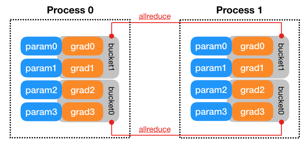
Another detail in [2] is how gradient synchronization is started in the backward phase. It says that “DDP uses autograd hooks registered at construction time to trigger gradients synchronizations. “
I did a quick experiment to verify these design details. test_multi_gpu is in charge of spawning worker processes and the real model training happens in the _worker function. initialize_trainer is the piece of code for initializing models at each process. Check out my comment in “Logs” section in the pseudocode below for the explanation for DPP’s behavior.
def test_multi_gpu(
    use_gpu: bool,
    num_gpus: int,
    normalization_data_map: Dict[str, NormalizationData],
    reader_options: ReaderOptions,
):
    logger.info(f"Enter test_multi_gpu with reader options {reader_options}")

    # These ENVS are needed by torch.distributed: https://fburl.com/1i86h2yg
    os.environ["MASTER_ADDR"] = "127.0.0.1"
    os.environ["MASTER_PORT"] = str(find_unused_port())

    manager = mp.Manager()
    result_dict = manager.dict()

    workflow_run_id = flow.get_flow_environ().workflow_run_id
    # The second condition is to avoid collision in unit test.
    # When running unit test, a local DB is used.
    # As a result, the workflow run ID may not be unique.
    if workflow_run_id and workflow_run_id > 10000:
        init_method = f"zeus://{workflow_run_id}"
    else:
        host_name = socket.gethostname()
        process_id = os.getpid()
        init_method = f"zeus://{host_name}_{process_id}"

    backend = "nccl" if use_gpu else "gloo"

    mp.spawn(
        _worker,
        args=(
            use_gpu,
            num_gpus,
            backend,
            init_method,
            reader_options,
            normalization_data_map,
            result_dict,
        ),
        nprocs=num_gpus,
        join=True,
    )
    logger.info("finish spawn")


def _worker(
    rank: int,
    use_gpu: bool,
    world_size: int,
    backend: str,
    init_method: str,
    reader_options: ReaderOptions,
    normalization_data_map: Dict[str, NormalizationData],
    reward_options: Optional[RewardOptions] = None,
    warmstart_path: Optional[str] = None,
    output_dict=None,
):
    logger.info(f"rank={rank} with reader options {reader_options}")
    dist.init_process_group(
        backend=backend, init_method=init_method, world_size=world_size, rank=rank
    )
    if use_gpu:
        torch.cuda.set_device(rank)

    model = create_model(...)
    trainer = model.initialize_trainer(
        use_gpu=use_gpu,
        reward_options=reward_options,
        normalization_data_map=normalization_data_map,
        warmstart_path=warmstart_path,
    )
    logger.info(f"rank={rank} finish initialize")

    num_of_data = 0
    data_reader = construct_distributed_data_reader(
        normalization_data_map, reader_options
    )
    for idx, batch in enumerate(data_reader):
        batch = post_data_loader_preprocessor(batch)
        if use_gpu:
            batch = batch.cuda()

        num_of_data += len(batch.training_input.state.float_features)

        logger.info(
            f"rank={rank} batch state={batch.training_input.state.float_features}"
        )
        logger.info(
            f"rank={rank} before train seq2slate param={print_param(trainer.seq2slate_net.seq2slate_net.seq2slate)}"
        )
        if rank == 1:
            logger.info(f"rank={rank} wake")
            time.sleep(60)
            logger.info(f"rank={rank} sleep")

        trainer.train(batch)
        logger.info(
            f"rank={rank} after train seq2slate param={print_param(trainer.seq2slate_net.seq2slate_net.seq2slate)}"
        )

        break

    logger.info(f"rank={rank} finish reading {num_of_data} data")


def initialize_trainer(self) -> Seq2SlateTrainer:
    seq2slate_net = initialize_model(...)

    if self.use_gpu:
        seq2slate_net = seq2slate_net.cuda()

    logger.info(f"Within manager {print_param(seq2slate_net.seq2slate)}")
    logger.info(
        f"Within manager {next(seq2slate_net.seq2slate.parameters()).device}"
    )
    if self.trainer_param.num_parallel > 1:
        seq2slate_net = _DistributedSeq2SlateNet(seq2slate_net)

    return _initialize_trainer(seq2slate_net)

###############
     Logs
###############
# This is printed within manager.initialize_trainer to show that
# models are initially with different parameters
# (see line 66 then line 112~115):
I1003 063214.340 seq2slate_transformer.py:140] Within manager tensor([-0.2585,  0.3716, -0.1077, -0.2114,  0.1636,  0.1398, -0.2960, -0.1204,\n ...], device='cuda:0', grad_fn=<CatBackward>)
I1003 063214.341 seq2slate_transformer.py:142] Within manager cuda:0
I1003 063214.349 seq2slate_transformer.py:140] Within manager tensor([-0.1076, -0.0444,  0.3003, -0.1177,  0.0275, -0.0811,  0.2084,  0.3369,\n ...], device='cuda:1', grad_fn=<CatBackward>)


# Below is printed from line 85 ~ 90
# You can see that each process receives different, non-overlapping data
# You can also see that at this point, the two models have the same parameters,
# which are ensured by DDP. The parameters come from one particular copy (rank=0)
I1003 063214.531 test_multi_gpu.py:144] rank=0 batch state=tensor([[ 0.0000,  0.0000, -0.0000,  ..., -1.6131, -1.6298, -1.6118],\n ...]],\n       device='cuda:0')
I1003 063214.540 test_multi_gpu.py:147] rank=0 before train seq2slate param=tensor([-0.2585,  0.3716, -0.1077, -0.2114,  0.1636,  0.1398, -0.2960, -0.1204,\n
 ...], device='cuda:0', grad_fn=<CatBackward>)
I1003 063214.544 test_multi_gpu.py:144] rank=1 batch state=tensor([[ 0.0000,  0.0000, -0.7115,  ..., -2.2678, -2.3524, -2.4194],\n  ...]],\n       device='cuda:1')
I1003 063214.553 test_multi_gpu.py:147] rank=1 before train seq2slate param=tensor([-0.2585,  0.3716, -0.1077, -0.2114,  0.1636,  0.1398, -0.2960, -0.1204,\n         ..., device='cuda:1', grad_fn=<CatBackward>)


# We deliberately let rank 1 sleep for one minute.
# But you can see that rank 0 does not return from its train function earlier
# because it blocks on .backward function, waiting for rank 1's backward() finish.
# You can see after .train function, both processes have resulted to the same parameters again
I1003 063214.554 test_multi_gpu.py:150] rank=1 wake
I1003 063314.613 test_multi_gpu.py:152] rank=1 sleep
I1003 063315.023 seq2slate_trainer.py:181] 1 batch: ips_loss=-2.706389904022217, clamped_ips_loss=-2.706389904022217, baseline_loss=0.0, max_ips=27.303083419799805, mean_ips=0.6373803615570068, grad_update=True
I1003 063315.033 test_multi_gpu.py:156] rank=0 after train seq2slate param=tensor([-0.2485,  0.3616, -0.0977, -0.2214,  0.1736,  0.1298, -0.3060, -0.1304,\n         ...], device='cuda:0', grad_fn=<CatBackward>)
I1003 063315.033 test_multi_gpu.py:161] rank=0 finish reading 1024 data
I1003 063315.039 seq2slate_trainer.py:181] 1 batch: ips_loss=-2.7534916400909424, clamped_ips_loss=-2.7534916400909424, baseline_loss=0.0, max_ips=272.4482116699219, mean_ips=0.908729612827301, grad_update=True
I1003 063315.050 test_multi_gpu.py:156] rank=1 after train seq2slate param=tensor([-0.2485,  0.3616, -0.0977, -0.2214,  0.1736,  0.1298, -0.3060, -0.1304,\n         ...], device='cuda:1', grad_fn=<CatBackward>)
I1003 063315.050 test_multi_gpu.py:161] rank=1 finish reading 1024 data
References
[1] https://www.telesens.co/2019/04/04/distributed-data-parallel-training-using-pytorch-on-aws/
 (next state) is a function of
  (current state) and
  (action);
  (reward) is also a function of
  and
and  , you will find that
  is independent of
  while
while  is not independent of
  . See [5, 6]. The noise independence test can be done through kernel-based test (see reference in [6]). The only situation where this method cannot distinguish the causal direction is when X and Y have a linear relationship and their noise is Gaussian. The second method is related to the Kolmogorov complexity. Theorem 1 from [7] states that under some assumptions if X->Y then
  , which can be proxied as so called pinball loss. Then quantile regression (regression using pinball loss) can be fitted for X to Y and Y to X. The direction with lower pinball loss would indicate the causal relationship. The third method is called matching. While there are several methods for matching, we talk about a widely adopted one called propensity score matching. The idea is that you group events together with similar propensity scores. The propensity score of an event is how likely it happens. Once similarly likely events are grouped together, you can further divide them by whether they receive some “treatment” and compute causal effect. One good example of applying propensity score matching is from an NLP work [11] where they probe which word causes positive or negative emotions. Some people criticize propensity score matching for its drawbacks [9, 10] and there are more matching methods to be considered [10]. We need to be very careful about the assumptions of these methods, since many of them cannot work when confounding variables are present.
  lies within the predicted interval
 ![[y_l, y_u]](https://czxttkl.com/wp-content/ql-cache/quicklatex.com-27d4a8ffbaed137ccc15f962a9474686_l3.png "Rendered by QuickLaTeX.com") .
.

 This means at any time of A2C all workers and the global network always have the same parameters. Of course, the drawback of A2C is that the speed of one global gradient update is determined by the slowest worker.
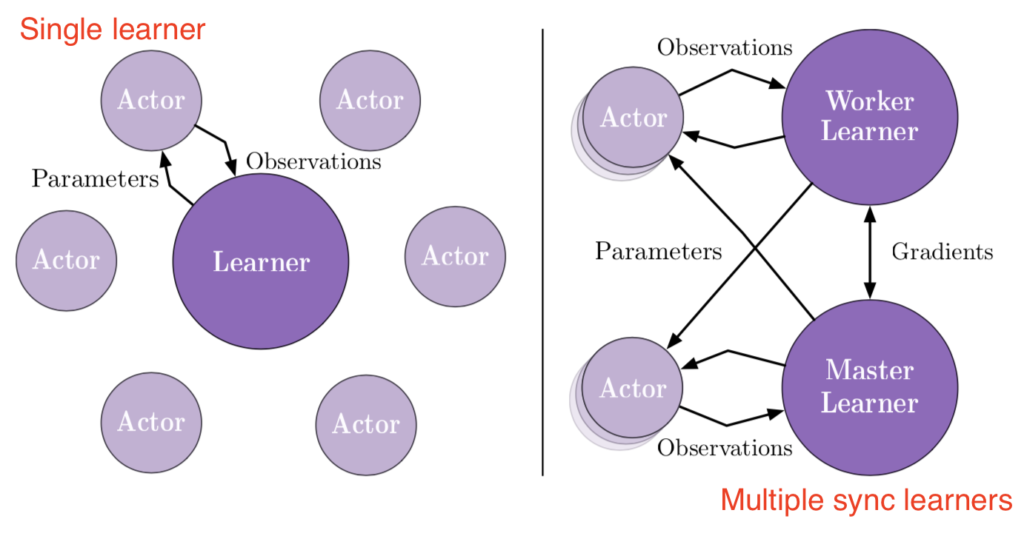
 and
and  in [2]:
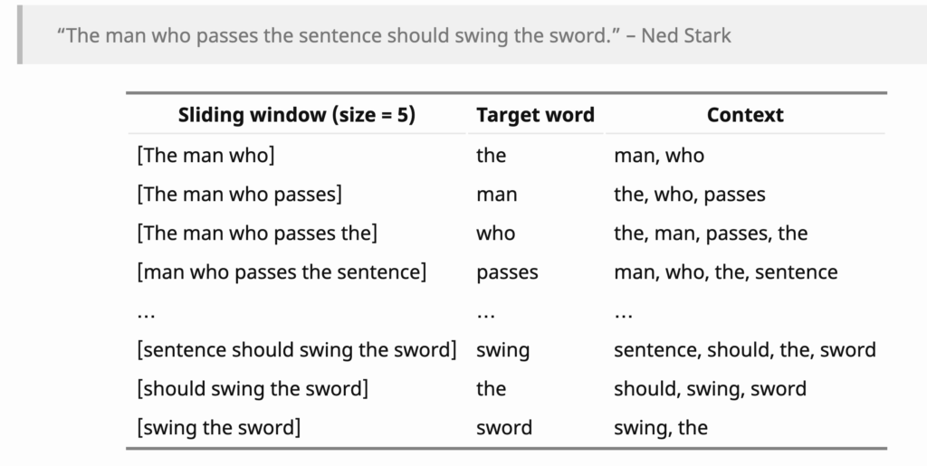
 :
:
 is a scoring function to score the similarity of any pair
  comes from all other possible words in the entire vocabulary. Obviously, this can be an expensive loss function if the vocabulary size is large, which is usually the case.
  additional words from the vocabulary to form a negative sample set. Among the k+1 words (
 provided
  at least one out of
  words:
 should be as high as possible; for the word
  should be as high as possible. That is what Eqn. 8 from [2] is about:
![\begin{equation*} J^h(\theta) = \mathbb{E}_{w \in (w,h)} \left[ log P^h(D=1|w,\theta)\right] + k \mathbb{E}_{w \not\in (w,h)} \left[ log P^h(D=0|w,\theta) \right]\end{equation*}](https://czxttkl.com/wp-content/ql-cache/quicklatex.com-3921a7faf12f5c8702e98f43bfa4f035_l3.png "Rendered by QuickLaTeX.com")
 . With the replacement, we won’t need to worry about how to compute the partition function
  as in Eqn.
 ![\mathbb{E}_{p(x)}[f(x)]](https://czxttkl.com/wp-content/ql-cache/quicklatex.com-c90b259513baa02e344aa8367f8c223d_l3.png "Rendered by QuickLaTeX.com") by Monte Carlo samples, we can instead evaluate
by Monte Carlo samples, we can instead evaluate ![\mathbb{E}_{p(x)}[f(x)-h(x)+\theta]](https://czxttkl.com/wp-content/ql-cache/quicklatex.com-b13a4b8be64daf2c070d7f4c57fd8a3a_l3.png "Rendered by QuickLaTeX.com") with
with ![\theta=\mathbb{E}_{p(x)}[h(x)]](https://czxttkl.com/wp-content/ql-cache/quicklatex.com-a8de21a662a2a66494d54b9acdc51880_l3.png "Rendered by QuickLaTeX.com") in order to reduce variance. The requirement for control variate to work is that
in order to reduce variance. The requirement for control variate to work is that  is correlated with
  and the mean of
  . Therefore, if we pick the second order of Taylor expansion for
  , we get
  .
. ![f(u_1, u_2)=exp[(u_1^2 + u_2^2)/2]](https://czxttkl.com/wp-content/ql-cache/quicklatex.com-f69a56e44acd47bc30c23e01cc063e79_l3.png "Rendered by QuickLaTeX.com") and we want to evaluate the integral
and we want to evaluate the integral  . If we want to use Monte Carlo estimator to estimate
  using
using  samples, we have:
 (we use multi-variable Taylor expansion here [7]). We first compute its mean:
 ![\theta=\mathbb{E}_{p(x)}[h(x)] = \int^1_0\int^1_0 \left(1 +(u_1^2+u_2^2)/2 \right) du_1 du_2 = 4/3](https://czxttkl.com/wp-content/ql-cache/quicklatex.com-78f185df22133a668d294ba879d7e49f_l3.png "Rendered by QuickLaTeX.com") . Thus, our control variate Monto Carlo estimator is:
. Thus, our control variate Monto Carlo estimator is:![\frac{1}{m}\sum\limits_{k=1}^{m} z(u_1, u_2)\newline=\frac{1}{m}\sum\limits_{k=1}^{m} \left[f(u_1, u_2) -h(u_1, u_2) + \theta\right]\newline=\frac{1}{m}\sum\limits_{k=1}^{m} \left[exp[(u_1^2 + u_2^2)/2] - 1 - (u_1^2 + u_2^2)/2 + 4/3 \right]](https://czxttkl.com/wp-content/ql-cache/quicklatex.com-cefe400b6090655af28e4c28735815f6_l3.png "Rendered by QuickLaTeX.com") .
. is smaller than
  .
.
![\nabla_\theta J(\theta) = \mathbb{E}_{s_t \sim \rho_{\pi}(\cdot), a_t \sim \pi(\cdot | s_t)} \left[ \nabla_\theta log \pi_\theta (a_t | s_t) R_t\right]](https://czxttkl.com/wp-content/ql-cache/quicklatex.com-837adae19f5b171b2c9a7a93a089f8ff_l3.png "Rendered by QuickLaTeX.com")
 to approximate
  , which causes variance. If we have a control variate
  and
and  can be chosen at any value but a sensible choice being
  , a deterministic version of
  , then the control variate version of policy gradient can be written as (Eqn. 7 in [2]):
![\nabla_\theta log \pi_\theta(a_t | s_t) R_t - h(s_t, a_t) + \mathbb{E}_{s\sim \rho_\pi, a \sim \pi}\left[ h(s_t, a_t)\right] \newline=\nabla_\theta log \pi_\theta(a_t | s_t) R_t - h(s_t, a_t) + \mathbb{E}_{s \sim \rho_\pi}\left[ \nabla_a Q_w(s_t, a)|_{a=\mu_\theta(s_t)} \nabla_\theta \mu_\theta(s_t)\right]](https://czxttkl.com/wp-content/ql-cache/quicklatex.com-9629b8ff4fc66089624196ff0d65190c_l3.png "Rendered by QuickLaTeX.com")
 is some critic with known analytic expression, and actually does not depend on
  .
.  , variance of actions
  , and variance of trajectories
  . What [3] highlights is that the magnitude of
  sends its i-th chunk to the next worker (with index
  ), and receives the (i-1)-th chunk from the previous worker. The received (i-1)-th chunk will be aggregated locally with the worker’s own (i-1)-th chunk. In the second cycle, each worker sends its (i-1)-th chunk, which got aggregated in the last cycle, to the next worker, and receives (i-2)-th chunk from the previous worker. Similarly, each worker now can aggregate on its (i-2)-th chunk with the received chunk which also indexes on i-2. Continuing on this pattern, each worker will send its (i-2), (i-3)-th, …chunk in each cycle until
  data aggregating cycles are done. Upon then each worker has one chunk that has been fully aggregated with all other workers. Then doing the similar circular cycles P-1 times can make all workers sync on all fully aggregated chunks from each other.
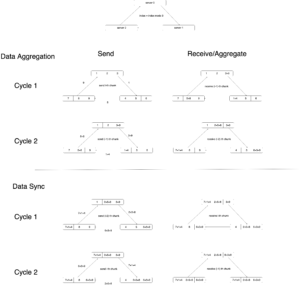
 is
is  . The gradient is a vector and can only be known fully when given a concrete value
  . The directional derivative is the gradient’s projection on another unit vector
  :
:  , where
  is inner product. See some introduction in [9] and [10].
 for all
  for some
  is convex on
  iff
iff  . Remember that
  is the change of
  caused by a tiny change in
  and we have
  .
.  .
.  , as long as
  is positive semidefinite, then
  with
with  ,
,  is all affine combinations of the vectors in
  , i.e.,
  .
. a subset of
  , the relative interior of
  . There is a good example from [8] which explains the difference between interior and relative interior.


 for the primal problem is defined as:
 , where
  (i.e.,
  ) and
) and  .
. is a local minimum of
 and
and 


 , and the objective function
  are convex, then KKT conditions also imply
  is defined as:


 (thus minimize
  , a convex function), and the constraints
  are convex. In a number of practical situations, the dual function
  and the minimum of the primal problem is
  . We have weak duality that always holds:
  . Strong duality holds when the dual gap is zero, with certain conditions holding, for example slater’s condition [14]. We can find the local minimum
  of the dual problem by a special form of gradient ascent algorithm called sequential optimization problem (SMO) [13] because special treatment is needed for the constraints involved in the dual problem.


 ,
, is a step size.


 , then we can iteratively update
  ,
,  , and
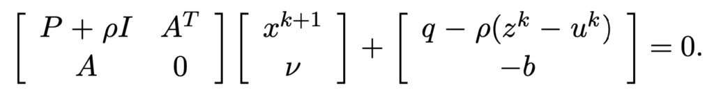
, and  separately, and such a method is called Alternating Direction Method of Multipliers (ADMM):


 as in the method of multipliers):


 and
and  , then the updates can be simplified as:


 ,
,  can often be exploited to carry out
  is an identity matrix,
  , and
, and  is the indicator function of a closed nonempty convex set
  , then
  , which means
  is the projection of
  onto
onto  and
and  becomes an unconstrained quadratic programming with the analytic solution at
  .
. and it must satisfy
  , then the ADMM primal problem becomes:
 (where
  is an indicator function of the nonnegative orthant
  )
)
 . This is a constrained quadratic programming. We have to use KKT conditions to solve it. Suppose the Lagrangian multiplier is
  , then the KKT conditions state that:
 ,
,
 ,
,  where
where 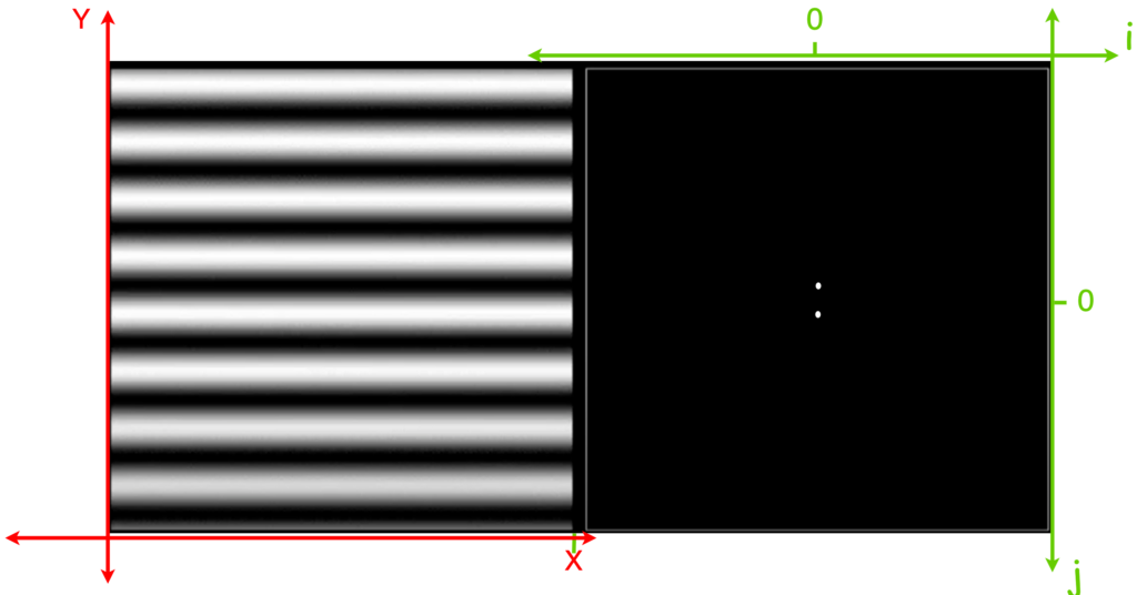
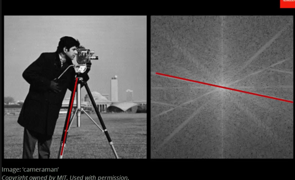
 -axis in frequency domain;
  -axis in the frequency domain. Because there is never fluctuation along the
  frequency. However, along the
  frequency. As a combination, we see two dots (two dirac delta functions) on the line
  because there is no signal variation on the
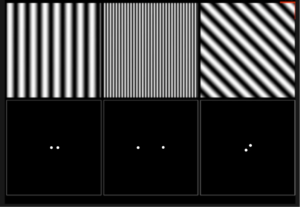
 (
(


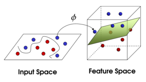
![\[K(\mathbf{x}, \mathbf{y})=exp\left(-\frac{\|\mathbf{x}-\mathbf{y}\|^2}{2\sigma^2}\right),\]](https://czxttkl.com/wp-content/ql-cache/quicklatex.com-b79b831a52476a21c48ca2567248e86f_l3.png "Rendered by QuickLaTeX.com")
 and
and  are two arbitrary points in the data space,
  is a hyperparameter of the Gaussian kernel that controls the sensitivity of difference when
  will be 1. The formula of Gaussian kernel is identical to the PDF of a normal distribution.
 and
and  ). The higher dimensional space is actually an infinite dimensional space, and the distance is measured by the dot product. That is,
  .
.
 data points
  with their labels
  . Each of the
  to the prediction of a new data point
  .
. 
 that are close to
  to denote the degree of
 . Therefore, we can solve the following matrix-vector equation to obtain
  :
:


![\[f(t)=(g*h)(t)=\int^\infty_{-\infty}g(\tau)h(t-\tau)d\tau\]](https://czxttkl.com/wp-content/ql-cache/quicklatex.com-237cc2257376e03764228a073433bafd_l3.png "Rendered by QuickLaTeX.com")
 , its frequency domain function
  is defined as:
![\[\hat{f}(\xi)=\int^{\infty}_{-\infty}f(t)e^{-2\pi i t \xi} dt\]](https://czxttkl.com/wp-content/ql-cache/quicklatex.com-bdcf4fbf82c13fb6b7e8c2a58a4ae12d_l3.png "Rendered by QuickLaTeX.com")
![\[f(t)=\int^\infty_{-\infty}\hat{f}(\xi)e^{2\pi i t \xi} d\xi\]](https://czxttkl.com/wp-content/ql-cache/quicklatex.com-1c2eeeb000305a965a637e37ca7f52a0_l3.png "Rendered by QuickLaTeX.com")
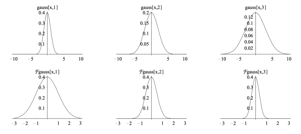
 , and suppose
  , and
, and  are the corresponding Fourier transformed functions. From the inverse Fourier transform we have
  and
and  .
.![(g*h)(t)=\int^\infty_{-\infty}g(\tau)h(t-\tau)d\tau \newline=\int^\infty_{-\infty} g(\tau)\left[\int^\infty_{-\infty} \hat{h}(\xi) 2^{\pi i (t-\tau) \xi}d\xi\right]d\tau \newline=\int^\infty_{-\infty} \hat{h}(\xi) \left[\int^\infty_{-\infty} g(\tau) 2^{\pi i (t-\tau) \xi}d\xi\right]d\tau \quad \quad \text{swap } g(\tau)\text{ and }\hat{h}(\xi)\newline=\int^\infty_{-\infty} \hat{h}(\xi) \left[\int^\infty_{-\infty} g(\tau) 2^{-\pi i \tau \xi} d\tau\right] 2^{\pi i t \xi} d\xi\newline=\int^\infty_{-\infty} \hat{h}(\xi) \hat{g}(\xi) 2^{\pi i t \xi} d\xi \newline = IFT\left[\hat{h}(\xi) \hat{g}(\xi)\right] \quad\quad Q.E.D.](https://czxttkl.com/wp-content/ql-cache/quicklatex.com-1771258be13b140b77c42f636647fb99_l3.png "Rendered by QuickLaTeX.com")
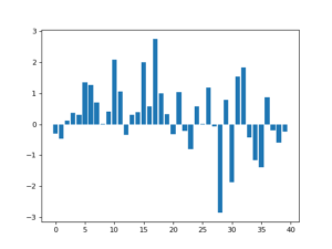
 with width 2 and height 1.
 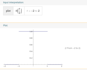 We know that its fourier transform is (
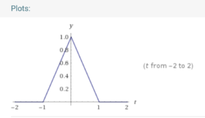
 , as we introduced in the application section, we probably get a smoother function roughly like a triangle function
  (
(
 ‘s fourier transform is (
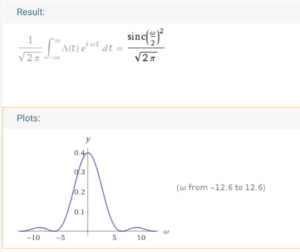
 .
.  is equal to
  . We know that
  function and
  would be attenuated.
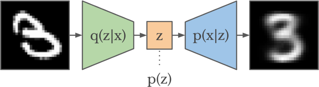
 . We’d like to use a parameterized distribution
  to approximate
  . To make
 ![\theta^* = argmin_\theta\; KL\left(q_\theta(z|x) || p(z|x) \right ) \newline= argmin_\theta \; \mathbb{E}_{q_\theta} [log\;q_\theta(z|x)] - \mathbb{E}_{q_\theta} [log\;p(z,x)]+log\;p(x)](https://czxttkl.com/wp-content/ql-cache/quicklatex.com-1acb87f9932eec25d3692cac471a68aa_l3.png "Rendered by QuickLaTeX.com")
![\mathbb{E}_{q_\theta}[f(z)]](https://czxttkl.com/wp-content/ql-cache/quicklatex.com-5525286df00a53261de88353c9e7658a_l3.png "Rendered by QuickLaTeX.com") means
means  , and
, and  is a constant w.r.t.
  and thus can be omitted. With simple re-arrangement, we can equivalently maximize the so-called ELBO function in order to find
  :
:![ELBO(\theta) \newline= \mathbb{E}_{q_\theta} [log\;p(z,x)] - \mathbb{E}_{q_\theta} [log\;q_\theta(z|x)]\newline=\mathbb{E}_{q_\theta}[log\;p(x|z)] + \mathbb{E}_{q_\theta}[log\;p(z)] - \mathbb{E}_{q_\theta}[log\;q_\theta(z|x)] \quad\quad p(z) \text{ is the prior of } z \newline= \mathbb{E}_{q_\theta}[log\;p(x|z)] - \mathbb{E}_{q_\theta} [log \frac{q_{\theta}(z|x)}{p(z)}]\newline=\mathbb{E}_{q_\theta}[log\;p(x|z)] - KL\left(q_\theta(z|x) || p(z)\right)](https://czxttkl.com/wp-content/ql-cache/quicklatex.com-8e4bcee52335d51120c9eb549e33fe95_l3.png "Rendered by QuickLaTeX.com")
 is also fitted by a parameterized function
  (this is the decoder of VAE). So the ultimate objective function we have for fitting a VAE is:
![\begin{equation*} $argmax_{\theta, \phi} \; \mathbb{E}_{x\sim D} \left[\mathbb{E}_{q_\theta}[log\;p_\phi(x|z)] - KL\left(q_\theta(z|x) || p(z)\right)\right]$\end{equation*}](https://czxttkl.com/wp-content/ql-cache/quicklatex.com-e113a0b22cbcbbbc91b73bf77605c0e6_l3.png "Rendered by QuickLaTeX.com")
![\mathbb{E}_{q_\theta}[log\;p_\phi(x|z)]](https://czxttkl.com/wp-content/ql-cache/quicklatex.com-cae4aa0a2d5f703241fac19b134f8aef_l3.png "Rendered by QuickLaTeX.com") can be thought as the so-called “reconstruction error”, which encourages the reconstructed
can be thought as the so-called “reconstruction error”, which encourages the reconstructed  encourages
  , then sample
 in Eq.
 . The gradient of Eq.
![\begin{align*}&\nabla_\theta \left\{\mathbb{E}_{q_\theta}[log\;p_\phi(x|z)] - KL\left(q_\theta(z|x) || p(z)\right)\right\}\\=&\nabla_\theta \left\{\mathbb{E}_{q_\theta}\left[log\;p_\phi(x, z) - \log q_\theta(z|x)\right] \right\} \quad\quad \text{ rewrite KL divergence} \\ =&\nabla_\theta \; \int q_\theta(z|x) \left[log\;p_\phi(x, z) - \log q_\theta(z|x) \right]dz \\=& \int \left[log\;p_\phi(x, z) - \log q_\theta(z|x) \right]\nabla_\theta q_\theta(z|x) dz + \int q_\theta(z|x) \nabla_\theta \left[log\;p_\phi(x, z) - \log q_\theta(z|x) \right] dz \\=& \mathbb{E}_{q_\theta}\left[ \left(log\;p_\phi(x, z) - \log q_\theta(z|x) \right) \nabla_\theta \log q_\theta(z|x) \right] + \mathbb{E}_{q_\theta}\left[\nabla_\theta \log p_\phi(x, z)\right] + \mathbb{E}_{q_\theta}\left[ \nabla_\theta \log q_\theta(z|x) \right] \\&\text{--- The second term is zero because no }\theta \text{ in } \log p_\phi(x,z) \\&\text{--- The third term being zero is a common trick. See Eqn. 5 in [1]} \\=& \mathbb{E}_{q_\theta}\left[ \left(log\;p_\phi(x, z) - \log q_\theta(z|x) \right) \nabla_\theta \log q_\theta(z|x) \right]\end{align*}](https://czxttkl.com/wp-content/ql-cache/quicklatex.com-ab36fc8bea2fc218505d19ee6e54e94c_l3.png "Rendered by QuickLaTeX.com")
 (
( is an independent source of noise):
![\begin{align*}&\nabla_\theta \left\{\mathbb{E}_{q_\theta}[log\;p_\phi(x|z)] - KL\left(q_\theta(z|x) || p(z)\right)\right\}\\=&\nabla_\theta \left\{\mathbb{E}_{q_\theta}\left[log\;p_\phi(x, z) - \log q_\theta(z|x)\right] \right\} \quad\quad \text{ rewrite KL divergence} \\=&\nabla_\theta \; \int q_\theta(z|x) \left[log\;p_\phi(x, z) - \log q_\theta(z|x) \right]dz \\=&\nabla_\theta \; \int p(\epsilon) \left[log\;p_\phi(x, z) - \log q_\theta(z|x) \right]d\epsilon \quad\quad \\&\text{--- Above uses the property of changing variables in probability density functions.} \\&\text{--- See discussion in [10, 11]} \\=& \int p(\epsilon) \nabla_\theta \left[log\;p_\phi(x, z) - \log q_\theta(z|x) \right]d\epsilon \\=& \int p(\epsilon) \nabla_z \left[log\;p_\phi(x, z) - \log q_\theta(z|x) \right] \nabla_\theta z d\epsilon \\=& \mathbb{E}_{p(\epsilon)} \left[ \nabla_z \left[log\;p_\phi(x, z) - \log q_\theta(z|x) \right] \nabla_\theta f_\theta(x) \right]\end{align*}](https://czxttkl.com/wp-content/ql-cache/quicklatex.com-4fafc4bcaae654c035173052feaa8981_l3.png "Rendered by QuickLaTeX.com")
 classes with class probability
  , which can be parameterized by a neural network consuming the raw data. There are several steps to perform the Gumbel-Softmax trick. First,
 ![\begin{align*}\arg\max_i \left[ g_i + log \pi_i \right]\end{align*}](https://czxttkl.com/wp-content/ql-cache/quicklatex.com-e0bca8c8b12be82c3fe266e5e8121352_l3.png "Rendered by QuickLaTeX.com")
 , with each component as:
 are i.i.d. samples drawn from
  distribution, and
  will be annealed through the training such that
  on
on  .
.  . Analytically,
 ![\mathbb{E}_{p(x)}[f(x)] = \int p(x)f(x)dx](https://czxttkl.com/wp-content/ql-cache/quicklatex.com-87f0b6db59bfd54a64b28bfa53049f7a_l3.png "Rendered by QuickLaTeX.com") . You can also think of
. You can also think of ![\mathbb{E}_{p(x)}[f(x)] = \int q(x')x'dx'=\mathbb{E}_{q(x')}[x']](https://czxttkl.com/wp-content/ql-cache/quicklatex.com-4e34970fdeef3ae11ba7c74589259884_l3.png "Rendered by QuickLaTeX.com") , the expectation of another random variable
, the expectation of another random variable  with any function exerted on it. Since I like the form
 ![\mathbb{E}_{p(x)}[f(x)]\approx \frac{1}{N}\sum\limits_{i=1}^Nf(x_i)](https://czxttkl.com/wp-content/ql-cache/quicklatex.com-6cea83b1e26813296576c469c343b9b0_l3.png "Rendered by QuickLaTeX.com")
 which can be seen as another random variable, is an unbiased estimate of
![\mathbb{E}_{p(x)}[z(x)]\newline=\mathbb{E}_{p(x)}[f(x)]-\mathbb{E}_{p(x)}[h(x)] + \theta\newline=\mathbb{E}_{p(x)}[f(x)]-\theta + \theta\newline=\mathbb{E}_{p(x)}[f(x)]](https://czxttkl.com/wp-content/ql-cache/quicklatex.com-119a2e3969f356586cea4c664bcffc85_l3.png "Rendered by QuickLaTeX.com")
![Var_{p(x)}[z(x)] \newline = Var_{p(x)}\left[f(x) - h(x)+\theta\right] \newline = Var_{p(x)}\left[f(x)-h(x)\right] \quad \quad \text{constant doesn't contribute to variance}\newline=\mathbb{E}_{p(x)}\left[\left(f(x)-h(x)-\mathbb{E}_{p(x)}\left[f(x)-h(x)\right] \right)^2\right] \quad\quad Var(x)=\mathbb{E}[(x-\mathbb{E}(x))^2] \newline=\mathbb{E}_{p(x)}\left[\left( f(x)-\mathbb{E}_{p(x)}[f(x)] - \left(h(x)-\mathbb{E}_{p(x)}[h(x)]\right) \right)^2\right]\newline=\mathbb{E}_{p(x)}\left[\left(f(x)-\mathbb{E}_{p(x)}[f(x)]\right)^2\right] + \mathbb{E}_{p(x)}\left[\left(h(x)-\mathbb{E}_{p(x)}[h(x)]\right)^2\right] \newline - 2 * \mathbb{E}_{p(x)}\left[f(x)-\mathbb{E}_{p(x)}[f(x)]\right] * \mathbb{E}_{p(x)}\left[h(x)-\mathbb{E}_{p(x)}[h(x)]\right]\newline=Var_{p(x)}\left[f(x)\right]+Var_{p(x)}\left[h(x)\right] - 2 * Cov_{p(x)}\left[f(x), h(x)\right]](https://czxttkl.com/wp-content/ql-cache/quicklatex.com-0ccdbafc7e844065190f08449216de2b_l3.png "Rendered by QuickLaTeX.com")
![Var_{p(x)}\left[h(x)\right] - 2 * Cov_{p(x)}\left[f(x), h(x)\right]< 0](https://czxttkl.com/wp-content/ql-cache/quicklatex.com-71ada8888072e46c10d992fc916f5516_l3.png "Rendered by QuickLaTeX.com") , we will reduce the variance of the estimate
, we will reduce the variance of the estimate  in
in 
 . However, when
 ![Var_{p(x)}[z(x)] \newline=Var_{p(x)}\left[f(x)\right]+c^2 \cdot Var_{p(x)}\left[h(x)\right] + 2c * Cov_{p(x)}\left[f(x), h(x)\right]](https://czxttkl.com/wp-content/ql-cache/quicklatex.com-17bc7bdff9ac5e1ae313fbe74320b19d_l3.png "Rendered by QuickLaTeX.com") ,
,![c^*=-\frac{Cov_{p(x)}[f(x),h(x)]}{Var_{p(x)}[h(x)]}](https://czxttkl.com/wp-content/ql-cache/quicklatex.com-0bd88e8db46779b5f087aeb8bf7396be_l3.png "Rendered by QuickLaTeX.com")
 , the optimal variance of
 ![Var^*_{p(x)}[z(x)] \newline=Var_{p(x)}\left[f(x)\right] - \frac{\left(Cov_{p(x)}\left[f(x), h(x)\right] \right)^2}{Var_{p(x)}[h(x)]}\newline=\left(1-\left(Corr_{p(x)}\left[f(x),h(x)\right]\right)^2\right)Var_{p(x)}\left[f(x)\right] \quad\quad Corr(x,y)=Cov(x,y)/stdev(x)stdev(y)](https://czxttkl.com/wp-content/ql-cache/quicklatex.com-397f1651dac767c2187126a6a9a18978_l3.png "Rendered by QuickLaTeX.com")
![[0, 10]](https://czxttkl.com/wp-content/ql-cache/quicklatex.com-a7f987864e941ee55f3f763288c0153e_l3.png "Rendered by QuickLaTeX.com") ,
,  and
and  . Statistical quantities can be calculated as:
![\mathbb{E}_{p(x)}[f(x)]=\frac{100}{3}](https://czxttkl.com/wp-content/ql-cache/quicklatex.com-eeea708654cb405018db16937032dff6_l3.png "Rendered by QuickLaTeX.com")
![Var_{p(x)}[f(x)]=\frac{8000}{9}](https://czxttkl.com/wp-content/ql-cache/quicklatex.com-d30026c49c0553b36cb87cf7a7657067_l3.png "Rendered by QuickLaTeX.com")
![\mathbb{E}_{p(x)}[h(x)]=5](https://czxttkl.com/wp-content/ql-cache/quicklatex.com-9686ee04edb180b5f6e38f9ce04af013_l3.png "Rendered by QuickLaTeX.com")
![Var_{p(x)}[h(x)]=\frac{25}{3}](https://czxttkl.com/wp-content/ql-cache/quicklatex.com-c717208bd00c192ea186d5f46f7ec4c1_l3.png "Rendered by QuickLaTeX.com")
![Cov_{p(x)}\left[f(x), h(x)\right]=\frac{250}{3}](https://czxttkl.com/wp-content/ql-cache/quicklatex.com-067065055b0006df97e40e185dffa214_l3.png "Rendered by QuickLaTeX.com")
![Var_{p(x)}[z(x)] \newline =Var_{p(x)}\left[f(x)\right]+Var_{p(x)}\left[h(x)\right] - 2 * Cov_{p(x)}\left[f(x), h(x)\right]\newline =\frac{8000}{9} + \frac{25}{3}-\frac{2\cdot 250}{3}\newline=\frac{6575}{9}<Var_{p(x)}[f(x)]](https://czxttkl.com/wp-content/ql-cache/quicklatex.com-386cf1266b42bd8a666f8421d6b2e6c5_l3.png "Rendered by QuickLaTeX.com") .
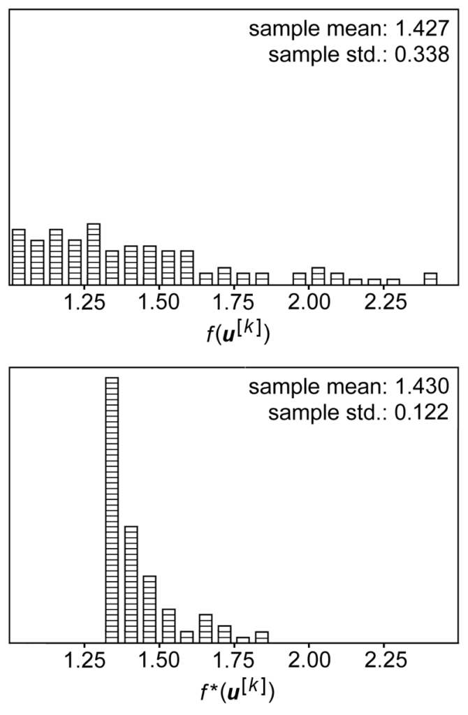
.![Var_{p(x)}[z(x)]](https://czxttkl.com/wp-content/ql-cache/quicklatex.com-173e2620e93733b9cab89fb86ad62e94_l3.png "Rendered by QuickLaTeX.com") with the assumption that it is a single-sample random variable. If we always collect
with the assumption that it is a single-sample random variable. If we always collect ![Var_{p(x)}[\bar{z}(x)]=Var_{p(x)}\left[\frac{\sum\limits_{i=1}^N z(x_i)}{N}\right]=N \cdot Var_{p(x)}\left[\frac{z(x)}{N}\right]=\frac{Var_{p(x)}\left[z(x)\right]}{N}](https://czxttkl.com/wp-content/ql-cache/quicklatex.com-8689d39a37054b16c04ad196608819f2_l3.png "Rendered by QuickLaTeX.com") . This matches with our intuition that the more samples you average over, the less variance you have. However, the relative ratio of variance you can save by introducing
. This matches with our intuition that the more samples you average over, the less variance you have. However, the relative ratio of variance you can save by introducing ![1-\left(Corr_{p(x)}\left[f(x),h(x)\right]\right)^2](https://czxttkl.com/wp-content/ql-cache/quicklatex.com-81740db5c9b00ddf2785429850fb97dd_l3.png "Rendered by QuickLaTeX.com") .
.