It has been some time since I got touch in neural architecture search (NAS) in my PhD, when I tried to get ideas for solving a combinatorial optimization problem for collectible card games’ deck recommendation. My memory about NAS mainly stays in one of the most classic NAS paper “Neural architecture search with reinforcement learning” [1], which uses policy gradient to search for better architectures. Apparently, things have advanced rapidly.
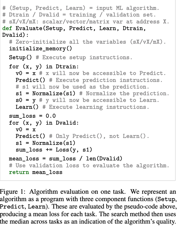
We can start from the most powerful NAS variant, AutoML-Zero [2]. It is not simply evolving an architecture, but actually evolve programs, literally. A program is defined with three main functions, setup(), learn(), and predict(). The algorithm uses evolutionary algorithms to search all possible implementations of the three functions using elementary operations. The objective of evolutionary algorithms is Evaluate() function shown below:
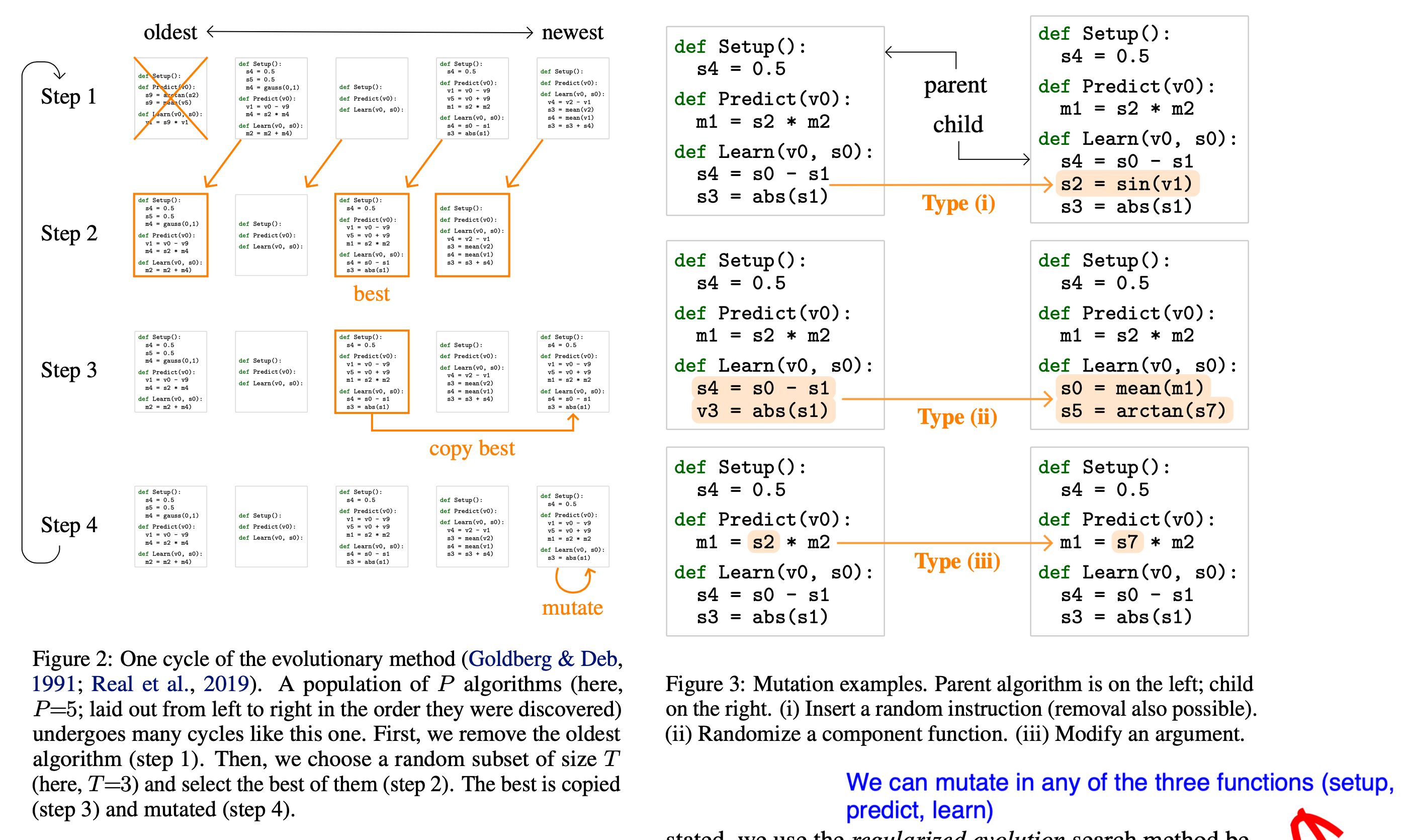
The evolutionary process is best illustrated in the following diagram:
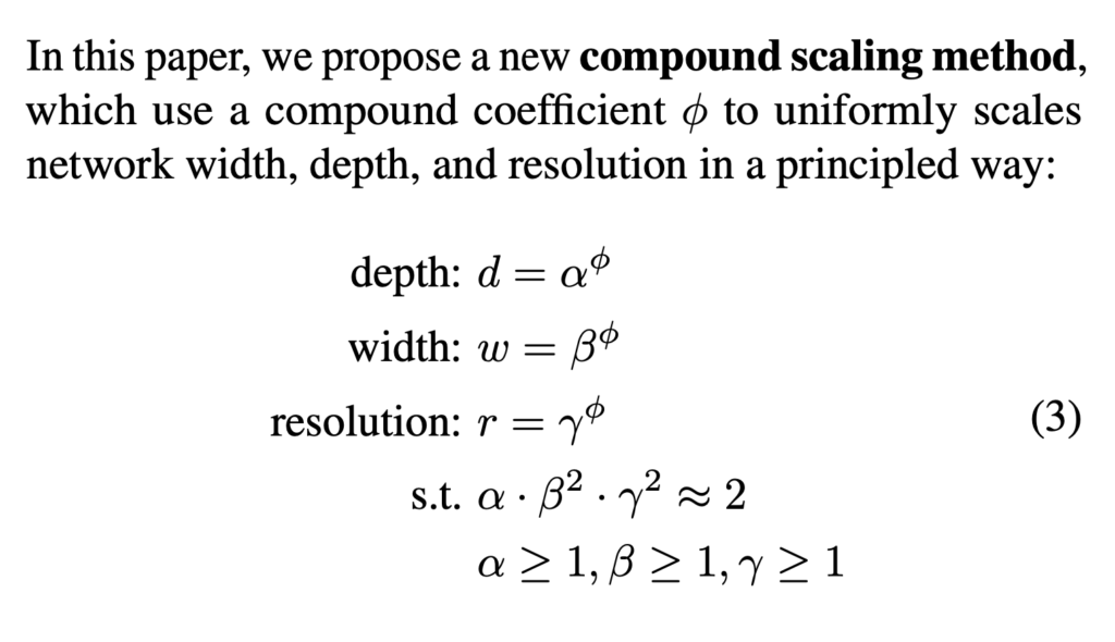
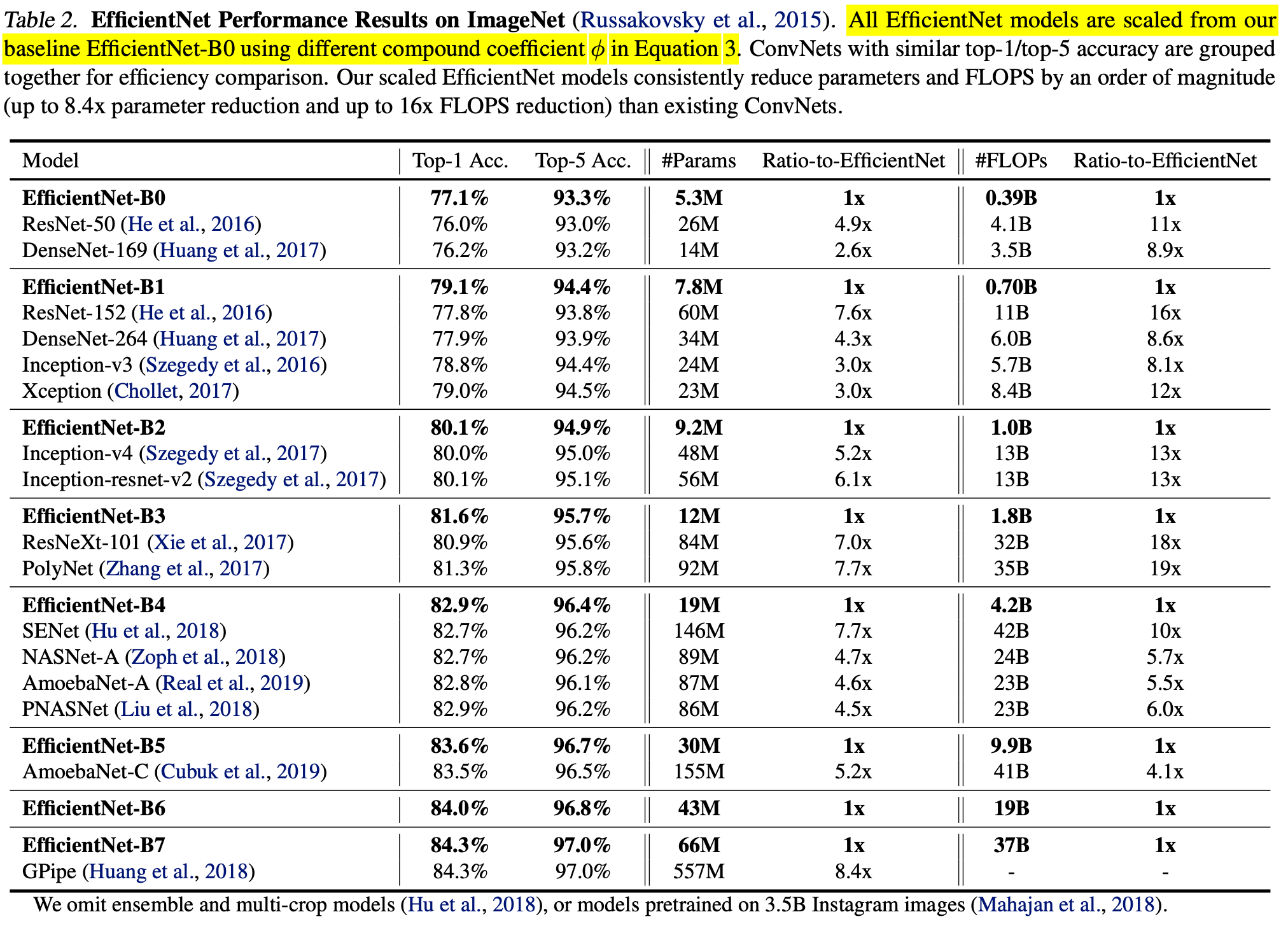
After seeing one of the most advanced NAS development, we can look at simpler ones. EfficientNet shows that deep neural networks can improve the most performance when depth, width, and resolution are scaled up simultaneously. This is a million-dollar-worth finding! Hence, they propose compound scaling, where they simply search over one dimension  :
:
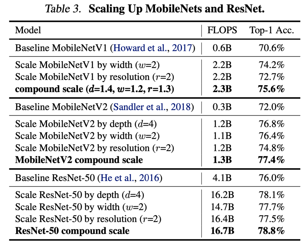
They show that scaling existing models like MobileNet and ResNet up lead to better performance then scaling one dimension (width, depth, resolution).
Next, they scale up a baseline model EfficientNet-B0, a model found by MnasNet [4]. As we can see, scaling up MnasNet leads to steady improvement in performance. MnasNet is also a policy gradient-based NAS algorithm, similar to earlier works like [1] (which might not be sample efficient). But it has two main improvements: (1) the reward adds latency penalty; (2) each block is repeating one sub-architectures and different blocks could have different sub-architectures; as comparison, previous works repeat only one sub-architectures in multiple blocks.
Besides EfficientNet, another simple yet effective method is using random search over a predictor that is trained on different possible architectures for predicting their performance (Neural Predictor from [5]). The predictor itself uses graph neural networks (specifically, graph convolutional network) to consume neural architectures represented as graphs. Most graph neural networks learn to represent node embeddings. However, in this work, they are interested in a regression model which maps the overall graph structure (architecture) to a scalar (performance), so they average the node embeddings to represent the overall graph’s embedding as the regression model’s input.
The ancestor of Neural Predictor is PNAS [9], which progressively expands architectures. At each step of expansion, it queries a trained predictor for which block to expand. The predictor is trained on (architecture of  blocks, performance), while it is used to predict the performance of architectures of
  blocks. PNAS cannot be fully parallelizable because of its progressive nature. That is one downside compared to Neural Predictor.
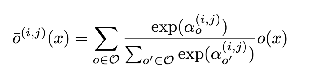
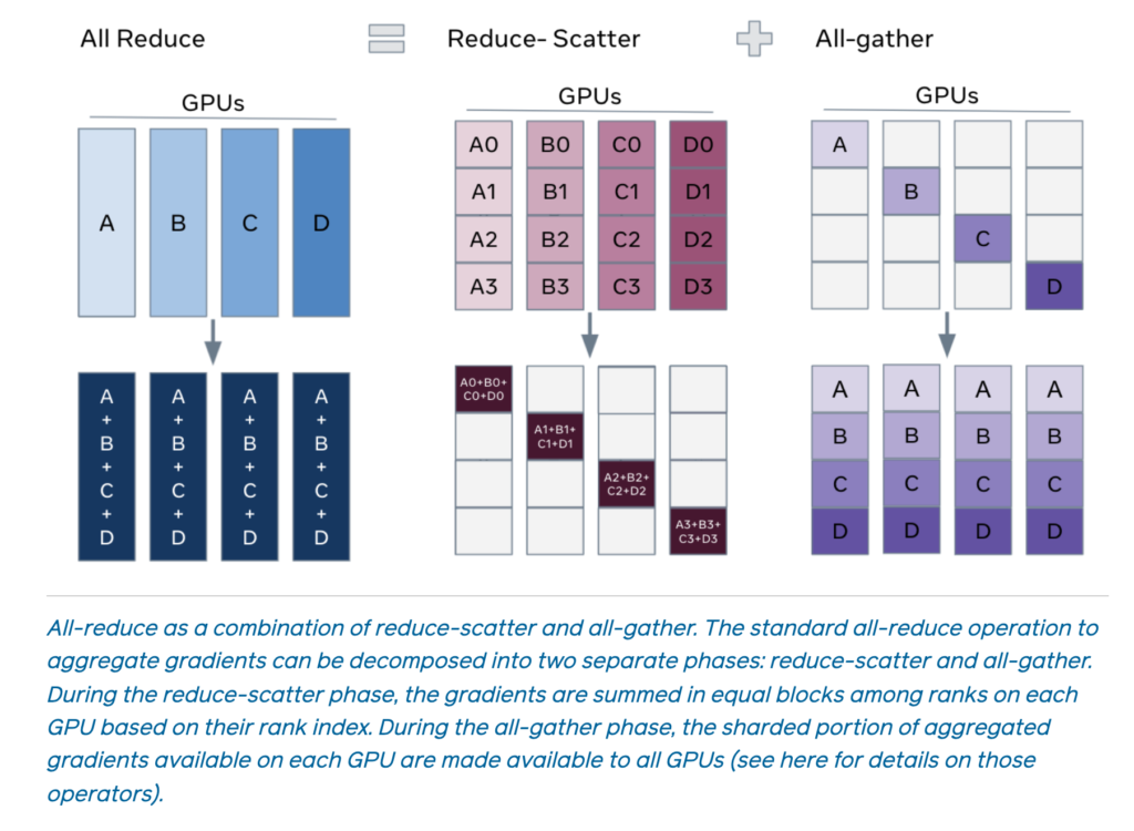
Now, let’s move on to one-shot NAS, which mostly revolve around the weight sharing technique. We use One-Shot [10], DARTS [11], and ProxylessNAS [8] to introduce the weight sharing technique. Weight sharing uses a much bigger architecture for training a model. The larger architecture covers all possible architectures we want to consider. If there are possible architectures  , then the output of One-Shot net and DARTS is (as summarized in ProxylessNAS [8]):
 , where
  in
in  is a softmax distribution over the architectures. To be clear, from the equation above, in order to compute
  or , we have to compute all the architectures’ outputs.
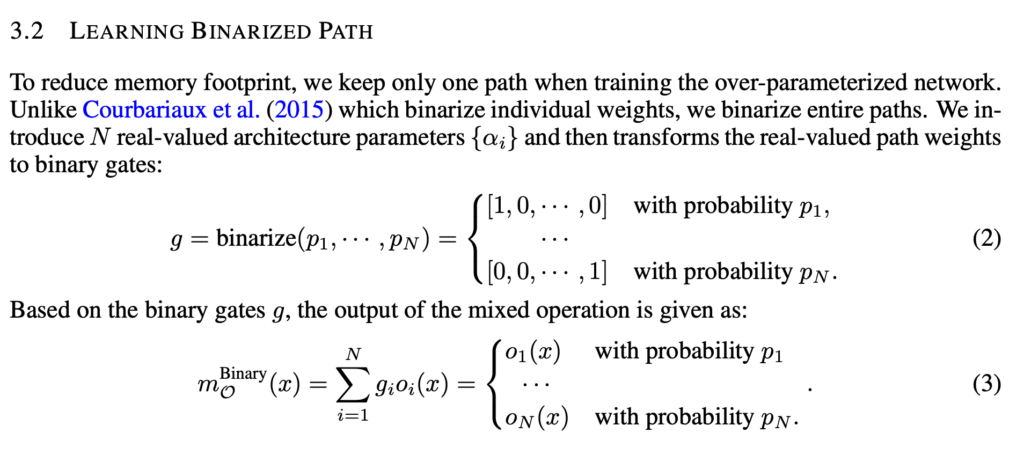
The problem with One-Shot and DARTS is that the memory needs to hold all architectures hence may easily blow up. ProxylessNAS proposes a technique called BinaryConnect, which is very close to DARTS but has subtle difference. BinaryConnect means that  , where
  is sampled from a softmax distribution. The difference with DARTS is that
  is strictly one architecture’s output, rather than a weighted sum of architectures. To take gradients of , they propose a trick to sample two architectures every time when computing the gradient:
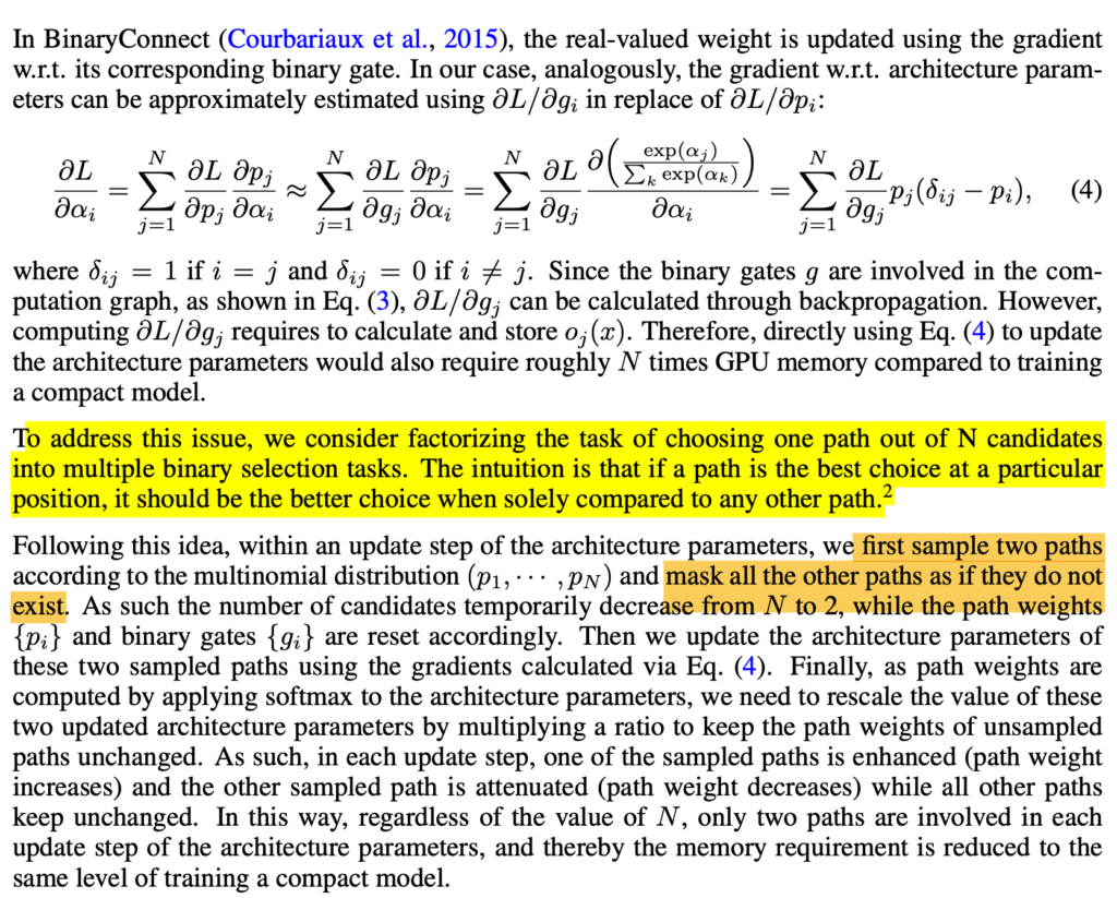
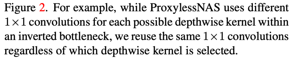
ProxylessNAS also proposes to train a neural network to predict latency so that model prediction accuracy and latency can be both differentiable w.r.t. architectures.
ENAS [12] is actually the originator of the weight sharing technique. One hurdle ENAS has over ProxylessNAS is that it requires an additional RNN controller to decide which architecture to sample. ProxylessNAS only needs to learn the softmax distribution parameters .
TuNAS [6] can be seen as an improved version over ProxylessNAS. There are mainly two improvements:
(1) more aggressive weight sharing, which they called operation collapsing.
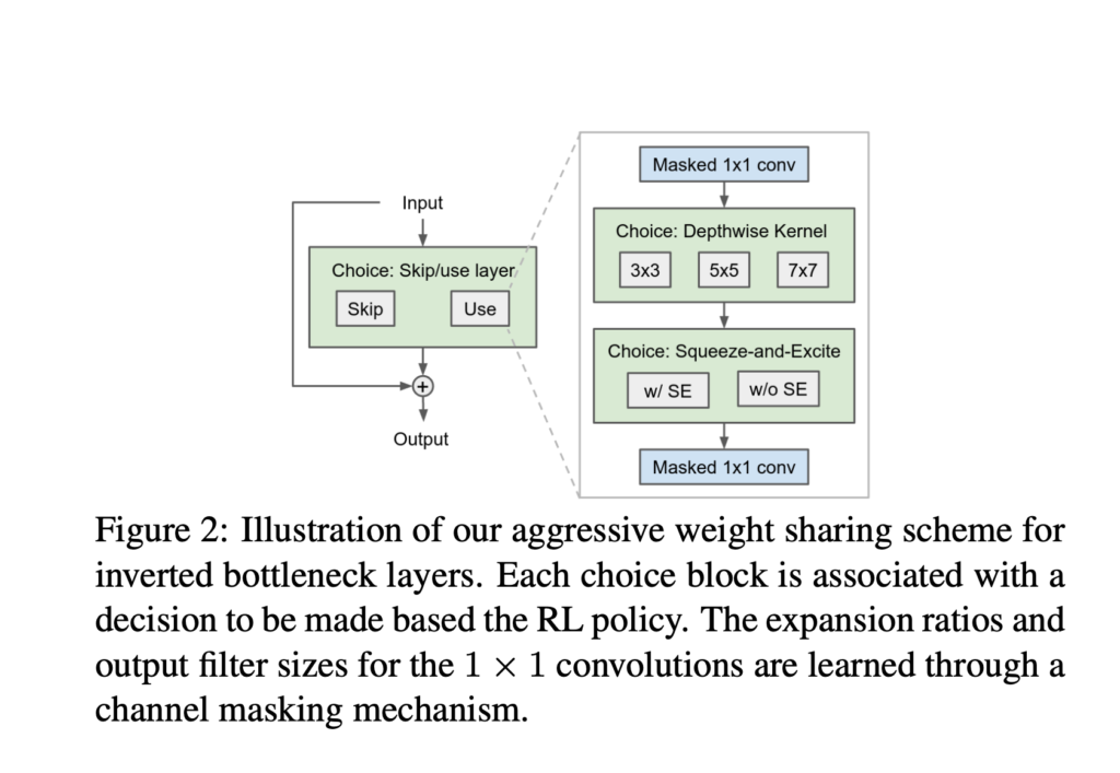
(2) a new reward function, which they claim leads to more robust results:
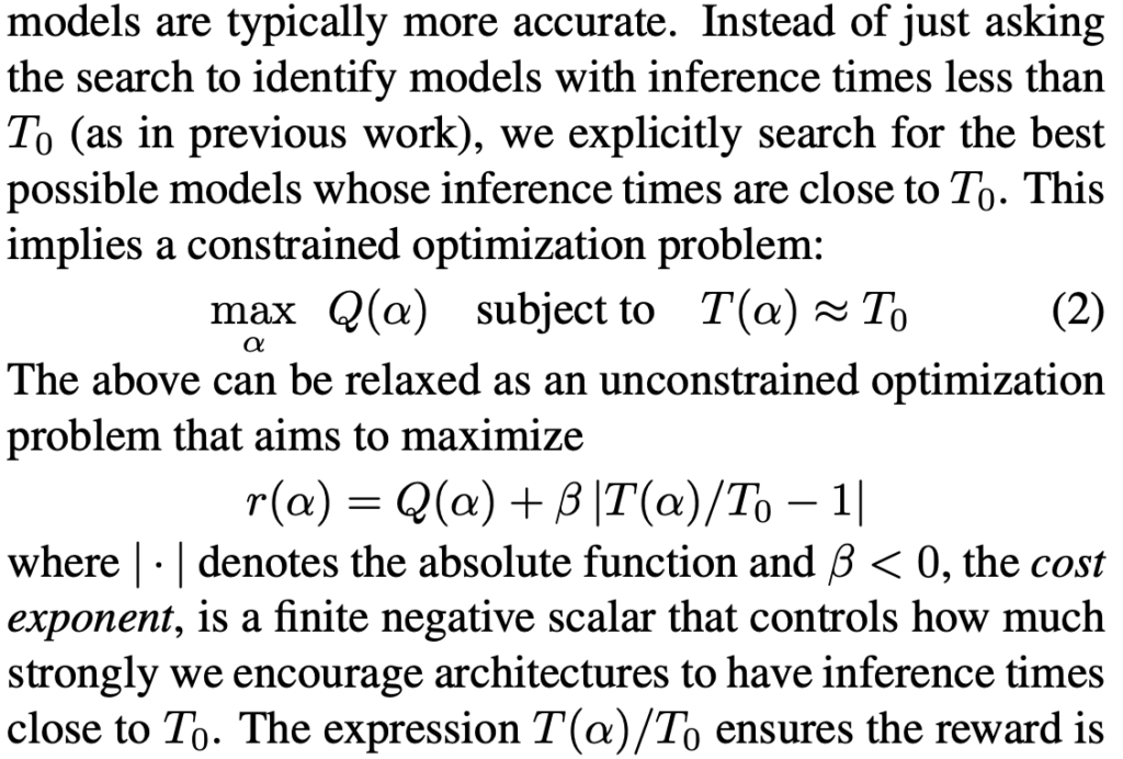
In TuNAS, policy gradient is used for sampling potential architectures, while weight sharing updates the sampled architectures’ weights. As the RL policy samples more and more architectures which cover all possible weights, all the weights in the biggest architecture get learned well. The overall learning loop is described as:

However, one problem arises from the weight sharing technique, as pointed out in the abstract of the BigNAS paper [7]: “existing methods assume that the weights must be retrained, fine-tuned, or otherwise post-processed after the search is completed”. BigNAS proposes several empirical tricks to make sure that architectures found by weight sharing can achieve good performance without retraining or post-processing steps. First, they introduce the sandwich rule, which samples the smallest child model, the biggest full model, and N randomly sampled child models. The gradients are aggregated from all the sampled models before relevant weights get updated. As [7] hypothesized, “The motivation is to improve all child models in our search space simultaneously, by pushing up both the performance lower bound (the smallest child model) and the performance upper bound (the biggest child model) across all child models.” Second, they introduce inplace distillation, which means the biggest full model’s prediction is used to supervise all child models through the whole training process. I am actually not sure why using the ground-truth labels for child models would be inferior than the teacher network’s prediction. Third, they design a learning rate schedule while ends up at a constant rather than simply exponentially decreasing. Moreover, they dedicate section 3.2 to describe a coarse-to-fine architecture selection paradigm after the full model is trained.
In parallel, few-shot NAS tries to solve a similar problem that evaluation based on the subnets sampled from a one-shot supernet usually have imperfect correlation with the evaluation based on those subnets retrained from scratch. So in few-shot NAS, multiple supernets are trained so that sampled subnets have better evaluation correlation. With less weight sharing than one-shot NAS but still lower computation than not using weight sharing, few-shot strikes a good balance. Please check [13] for more details.
In the last, I want to spend some time to specifically walk through some details from DARTS [11], SNAS [14], and DSNAS [15], which involves several advanced gradient-based methods to do one-shot learning.
In DARTS, as we survey when we introduce ProxylessNAS, the outcome of an input  is a softmax distribution over a set of candidate operators
  :
:
 then is a learnable vector determining which operator to be more preferable. Suppose the network’s own weight is
  , then the objective function of DARTS is essentially:
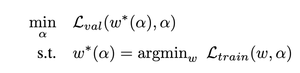 Note that is actually optimized on the validation dataset. As the paper suggests, this is a bi-level optimization problem. Analytically, the optimal solution is obtained when
  and
and  .
.
The paper proposes to replace  , the expensive minimization
  , with
  .
.
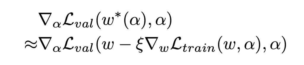
However, now and , the first and second argument in  , are both a function of , so we need to use the derivative rule of multi-variable functions to really compute
  . I refer to https://math.libretexts.org/Bookshelves/Calculus/Book%3A_Calculus_(OpenStax)/14%3A_Differentiation_of_Functions_of_Several_Variables/14.5%3A_The_Chain_Rule_for_Multivariable_Functions and https://www.programmersought.com/article/14295360685/#67_176 to really understand how to compute .
We use a simpler notation to represent  , where
  ,
,  ,
,  .
.
From the derivative rule of multi-variable functions
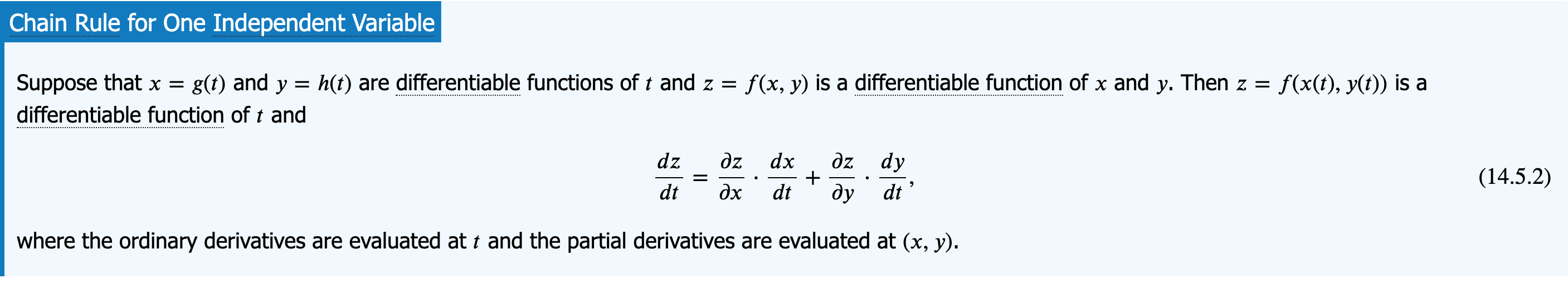
we have:

So we finally compute as:

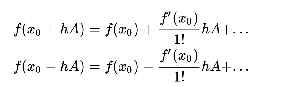
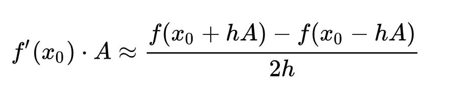
As you may notice,  is an expensive matrix-vector product, so people propose to use the finite difference approximation:

where 
The finite difference approximation is actually based on Taylor expansion:
The problem with DARTS is that after learning both the architecture selection parameter and the supernet’s own weight , it derives the best child network by  . As pointed out by SNAS [14], DARTS thus has “the inconsistency between the performance of derived child networks and converged parent networks”. SNAS uses the concrete distribution as the more principled way to learn the architecture selection parameter . In the concrete distribution, there is a parameter
  that will be annealed to be close to zero thus when the training finished, the architecture selection parameter will converge to discrete variables (clearly denoting which operator is connected between which pair of nodes).
The notations in the SNAS paper [14] is a bit chaotic. Hope I can comb them more cleanly. The idea of SNAS is that the architecture search parameter is a binary tensor  .
.  denotes the node
  is connected to node
  with operator
  . Therefore,
  is actually a one-hot encoding vector of length , i.e., the selection of one of the possible operators connecting node and . Similarly,
  is also a vector of length , denoting the output of the possible operators.

Therefore, the objective function of SNAS is:
![\begin{align*}\mathbb{E}_{\mathbf{Z} \sim p_\alpha(\mathbf{Z})}\left[\mathcal{L}_\theta(\mathbf{Z})\right],\end{align*}](https://czxttkl.com/wp-content/ql-cache/quicklatex.com-fe7b8d34da657b7c81c2d45efa42b0c2_l3.png "Rendered by QuickLaTeX.com")
where

is the model’s own loss.
Now, will be parameterized by the concrete distribution, which constitutes the parameter selection parameter  of the same size of , i.e.,
  , the Gumbel random variable
  , and the annealing parameter . Specifically,

The authors proves that ![\mathbb{E}_{\mathbf{Z} \sim p_\alpha(\mathbf{Z})}\left[\frac{\partial \mathcal{L}_\theta(\mathbf{Z})}{\partial \alpha_{i,j}^k}\right]](https://czxttkl.com/wp-content/ql-cache/quicklatex.com-9bc7133456ea15e95381b11e354287d0_l3.png "Rendered by QuickLaTeX.com") is essentially doing policy gradient.
is essentially doing policy gradient.
First, we make sure we are clear on the notations on how node ‘s input  interacts with other nodes that connect to it (small modification from equation 20 in [14]):

Now, using the chain rule of derivatives, we have
![\begin{align*}\begin{split}\frac{\partial \mathcal{L}_\theta(\mathbf{Z})}{\partial \alpha_{i,j}^k} &=\sum_{k'=1}^{K} \frac{\partial \mathcal{L}_\theta(\mathbf{Z})}{\partial x_j} \cdot \frac{\partial x_j}{\partial \mathbf{Z}_{i,j}^{k'}} \cdot \frac{\partial \mathbf{Z}_{i,j}^{k'}}{\partial \alpha_{i,j}^k} \\&=\sum_{k'=1}^{K} \frac{\partial \mathcal{L}_\theta(\mathbf{Z})}{\partial x_j} \cdot \mathbf{O}_{i,j}^{k'}(x_i) \cdot \frac{\partial \mathbf{Z}_{i,j}^{k'}}{\partial \alpha_{i,j}^k} \qquad\qquad (\text{replace } \frac{\partial x_j}{\partial \mathbf{Z}_{i,j}^{k'}}) \\&=\sum_{k'=1}^{K} \frac{\partial \mathcal{L}_\theta(\mathbf{Z})}{\partial x_j} \cdot \mathbf{O}_{i,j}^{k'}(x_i) \cdot \left(\left(\delta(k'-k)-\mathbf{Z}_{i,j}^{k'}\right)\mathbf{Z}_{i,j}^{k'}\frac{1}{\lambda \alpha_{i,j}^k}\right) \qquad(\text{replace } \frac{\partial x_j}{\partial \mathbf{Z}_{i,j}^{k'}}\text{ based on trick [16]})\end{split}\end{align*}](https://czxttkl.com/wp-content/ql-cache/quicklatex.com-9dab0d80fcafe83d0428f24f6ed7206e_l3.png "Rendered by QuickLaTeX.com")
Finally, Appendix D shows that:
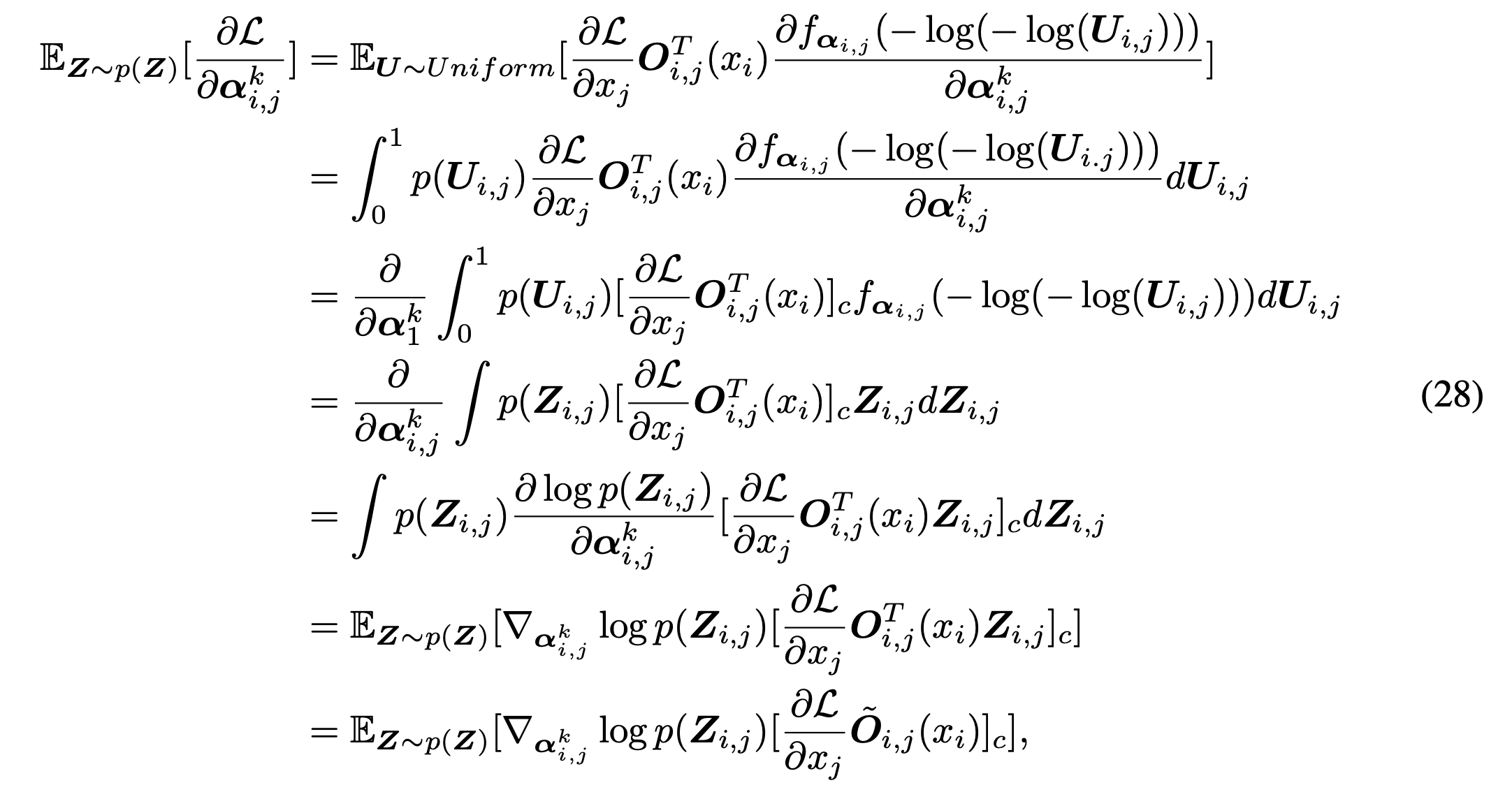
That’s the form of policy gradient. That’s why it is equivalent to say that SNAS is trained with policy gradient and with reward  .
.
I’ll dig into DSNAS [15] once it gets more attention.
——————– Update 2021/09 ——————–
I want to mention two more classic ideas of NAS.
- Regularized evolution [17], in which every mutated solution has a certain survival period. The only way that a good architecture can remain the population is by being passed down from parents to children through the generations. “regularized” means every solution has an age, therefore it encourages more diversity and exploration and avoids being stuck by spuriously promising solutions.
- Bayesian Optimization [18], in which there are five most important components: encoding, neural predictor, uncertainty estimate, acquisition function, and acquisition optimization. [18] used empirical experiments to find the optimal combination of them: path encoding (a specific feature engineering method they propose), an ensemble of 5 feedforward neural networks as uncertainty estimate, independent Thompson Sampling, and mutation-based acquisition optimization.
References (arxiv submitted time)
[1] NEURAL ARCHITECTURE SEARCH WITH REINFORCEMENT LEARNING (2016.11)
[2] AutoML-Zero: Evolving Machine Learning Algorithms From Scratch (2020.3)
[3] EfficientNet: Rethinking Model Scaling for Convolutional Neural Networks (2019.5)
[4] MnasNet: Platform-aware neural architecture search for mobile (2018.7)
[5] Neural Predictor for Neural Architecture Search (2019.12)
[6] Can weight sharing outperform random architecture search? An investigation with TuNAS (2020.8)
[7] BigNAS: Scaling Up Neural Architecture Search with Big Single-Stage Models (2020.3)
[8] ProxylessNAS: Direct Neural Architecture Search on Target Task and Hardware (2018.12)
[9] Progressive Neural Architecture Search (2017.12)
[10] Understanding and Simplifying One-Shot Architecture Search (2018)
[11] DARTS: Differentiable Architecture Search (2018. 6)
[12] Efficient Neural Architecture Search via Parameter Sharing (2018.2)
[13] Few-shot Neural Architecture Search (2020.6)
[14] SNAS: Stochastic Neural Architecture Search (2018.12)
[15] DSNAS: Direct Neural Architecture Search without Parameter Retraining (2020.2)
[16] softmax derivative trick https://eli.thegreenplace.net/2016/the-softmax-function-and-its-derivative/
[17] Regularized Evolution for Image Classier Architecture Search (2019.2)
[18] BANANAS: Bayesian Optimization with Neural Architectures for Neural Architecture Search (2020.11)
![\text{maximize}_{\theta} \quad \mathbb{E}_{x \sim P_{data}}\left[ P_{\theta}(x)\right],](https://czxttkl.com/wp-content/ql-cache/quicklatex.com-5fe9fcb62c0fc5ed93731b6ec6608093_l3.png "Rendered by QuickLaTeX.com")
 which has the highest likelihood for the data generated from the data distribution as such to “approximate” the data distribution.
  has an analytical form. Examples include Normalizing Flows, PixelCNN, PixelRNN, and WaveNet. The latter three examples are autoregressive models which generate elements (e.g., pixels, audio clips) sequentially however are computationally heavy due to the nature of autoregressive. Normalizing Flows can generate the whole image instantaneously thus has a computational advantage over others. (For more pros/cons of Normalizing Flows, please refer to [4])
 and
and  are random variables both with dimension
  . Also, suppose there is a mapping function
  such that
  and
and  . Then the density functions of
  ,
, . From now on, we assume that
  and
and  ), which is what we try to learn. The objective function for learning
 ). The reason that we want
  in the objective function so ideally
  should be easy to compute; second, once we learn
  and
and  , and then we can easily sample
  and apply
  to generate new data (e.g., new images). The requirement for a valid and practical
  or
or  is efficient to compute.
  to form a new transformation. Suppose
  with each
  having a tractable inverse and a tractable Jacobian determinant. Then:
 , where
  .
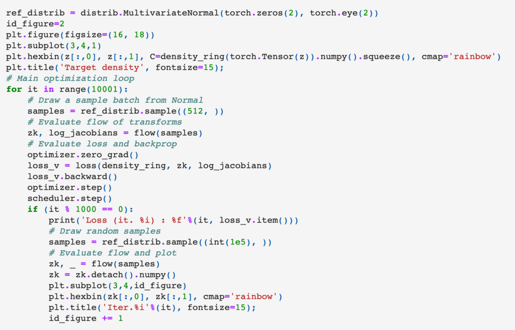
.  and optimize for log likelihood. Therefore, our objective becomes (as can be seen in Eqn. 1 from the Flow++ paper (one SOTA flow model) [5]):
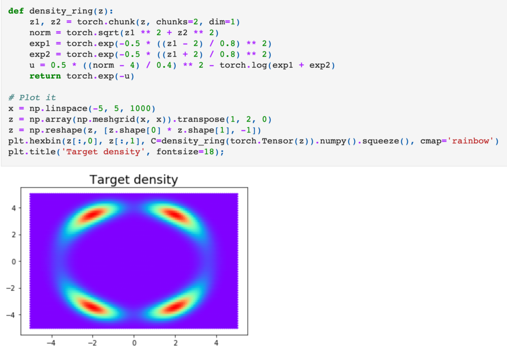 The objective function, as we already introduced above, is
  . Here,
  is the target
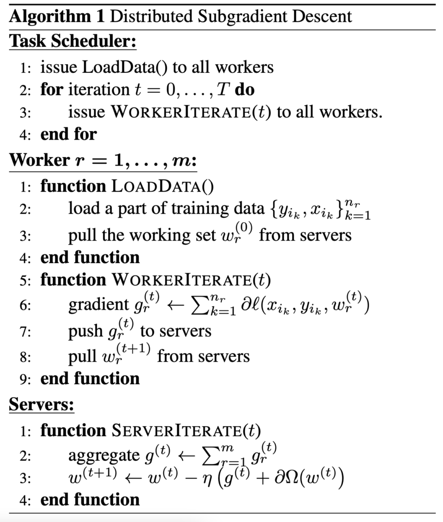


 GPUs, as shown in the table below, where
  ,
,  , and
, and  means we apply ZERO only on optimizer states, gradients, and parameters, respectively:
 is a learned critic function:
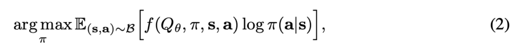
 . However, we can do much more than that choice:
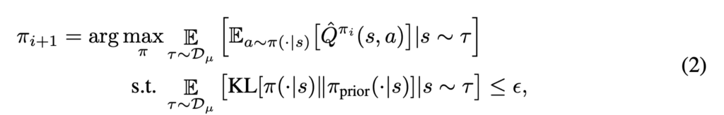

 is equal to the logging policy
  . So the optimal solution is supposed to be
  . The CRR paper points out it is equivalent to subtract the state value
  from
from  , leading to
  . (I am not sure how
  is omitted. )
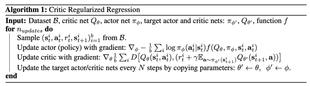


 using Eqn. 2. [2] provides two ways of optimization: (1) Expectation-Maximization, alternating between
  in the objective.
![\begin{align*}\begin{split}L&=\mathbb{E}_{s,a\sim D}\left[\delta(s,a)\right]\\&=\mathbb{E}_{s,a\sim D} \left[ \left\| Q(s,a) - \left(r(s,a) + \gamma max_{a'}Q(s',a') \right) \right\|^2 \right] \end{split}\end{align*}](https://czxttkl.com/wp-content/ql-cache/quicklatex.com-5aa31c8be06e51b513eb5a93f88c93ac_l3.png "Rendered by QuickLaTeX.com")
![\begin{align*}\begin{split}L&=\mathbb{E}_{s,a\sim D}\left[\delta(s,a)\right] + \alpha \cdot \mathbb{E}_{s\sim D, a \sim \pi} \left[ Q(s,a)\right],\end{split}\end{align*}](https://czxttkl.com/wp-content/ql-cache/quicklatex.com-e050be29b81a53dd71b71a2b907a363c_l3.png "Rendered by QuickLaTeX.com")
![\begin{align*}\begin{split}L&=\mathbb{E}_{s,a\sim D}\left[\delta(s,a)\right] + \alpha \cdot \left( \mathbb{E}_{s\sim D, a \sim \pi} \left[ Q(s,a)\right] - \mathbb{E}_{s,a \sim D} \left[ Q(s,a)\right] \right),\end{split}\end{align*}](https://czxttkl.com/wp-content/ql-cache/quicklatex.com-3fcda39c30f6eca37632bb2744d174b8_l3.png "Rendered by QuickLaTeX.com")

 For value iteration (they call MBS-QI):
 , which simply zeros out Q values of (state, action) frequency less than a threshold:
 , the count/probability distribution of encountering (state, action) pairs.
 , the lower bound of
  by
by  , where
  is an indicator function.
  on BCQ-updated Q-values to further zero out Q-values with less observed states.
  comes from a VAE trained only on state data.
 (encoding input
  ) and a generator
  (reconstructing the input based on
  and
and  entail the probability density of the latent vector and the reconstructed input. Usually,
  , where
  and
and  are the output of the encoder. VAE optimizes an objective function called ELBO (Evidence Lower Bound):
![ELBO(X) = \mathbb{E}_{z\sim\mathcal{E}(z|X)}\left[\log \mathcal{G}(X|z) \right] - D_{KL} \left[ \mathcal{E}(z|X) || P(z) \right] \leq \log\left[P(X)\right]](https://czxttkl.com/wp-content/ql-cache/quicklatex.com-fa96a09938c5043d068d83ba57b2ebf9_l3.png "Rendered by QuickLaTeX.com") .
. (as
(as  , then once this VAE is learned, you can compute ELBO for any test state
  , which can be interpreted as the lower bound of how likely
  denotes a condition vector:
![ELBO(X|C) = \mathbb{E}_{z\sim\mathcal{E}(z|X, C)}\left[\log \mathcal{G}(X|z, C) \right] - D_{KL} \left[ \mathcal{E}(z|X, C) || P(z) \right] \leq \log\left[P(X|C)\right]](https://czxttkl.com/wp-content/ql-cache/quicklatex.com-41062ec8c02785117194f9f3bd7f7f01_l3.png "Rendered by QuickLaTeX.com")
 where MMD is maximum mean discrepancy measuring the distance between two distributions using empirical samples:

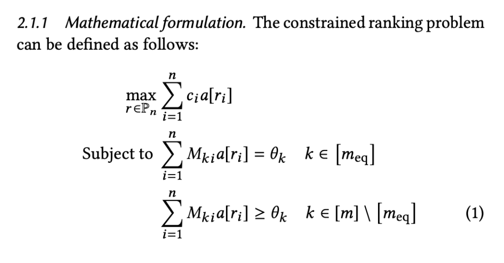
 is item
  is item
  , and
, and ![a[r_i]](https://czxttkl.com/wp-content/ql-cache/quicklatex.com-9384f0e69f08e8eb519cc02a63f47b63_l3.png "Rendered by QuickLaTeX.com") means the attention strength on each item when the item is ranked by
means the attention strength on each item when the item is ranked by  is the constraint matrix. As you can see, they define the slate reward/constraint as the sum of per-item rewards/constraints, which may or may not be the case for some application.
  possible rankings. Therefore, optimizing Eqn. 1 will be hard. They skillfully convert the problem into something more manageable. First, they rewrite Eqn. 1 into Eqn. 2:
 is a permutation matrix (each row and column has exactly one 1).
  , an “expected” permutation matrix. (In 3d, there is a typo. It should be
  ). Here,
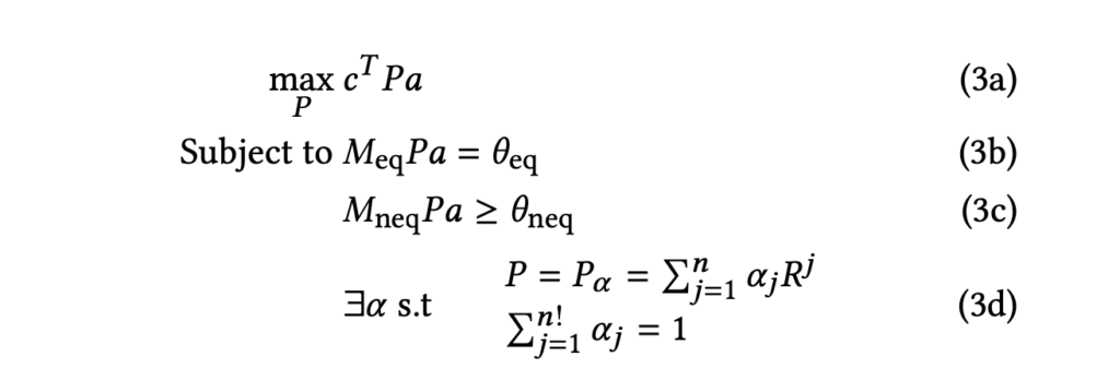
 entries:


 elements in an ads
  .
.  and
and  are the embeddings of a pair of elements, where the interaction score between the two embeddings could be computed using one of the operators, Concat, Multiply, Plus, Max, or Min. (mentioned in Section 4.2).
 ? We use stochastic variational inference (
 , how likely is to observe the current dataset?) and a KL divergence between the current Gaussian distribution and a prior Gaussian distribution, both of which have an analytical expression.
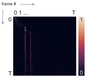
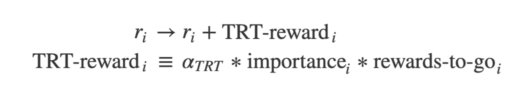
 The loss can be understood as that each step’s reward
  constitutes contribution from the current state
  and all previous states
  , gated by
  .
.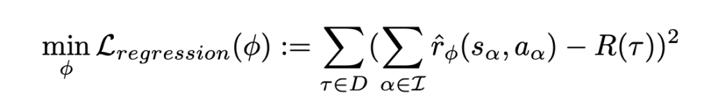 You can think of
  as
as  , i.e., the Transformers will take into accounts all previous steps until the current step to make the prediction of reward for the current step. The difference with [1] is that: a. [7] uses previous steps’ information more effectively using a sequence model; b. [7] only decomposes the total episode reward
  , while [1] decomposes for every step reward.
 As you can see, this environment could have
  states and only one state could give you a positive reward. It would almost be infeasible for a normal RL model to explore and learn effectively. What confused me but now is clear to me is that the state of this environment fed to an RL model has two parts, the current

 steps, they use a sequence model with attention mechanism to predict each pair of steps
  ‘s influence on reward (
 ). Specifically, the sequence model is a classifier predicting whether “the logit predicting whether the rewards-to-go from a given observation are below or above a threshold.” (from [9]).
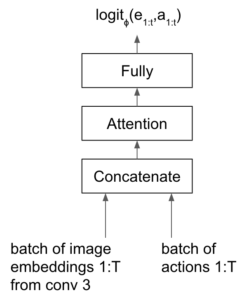


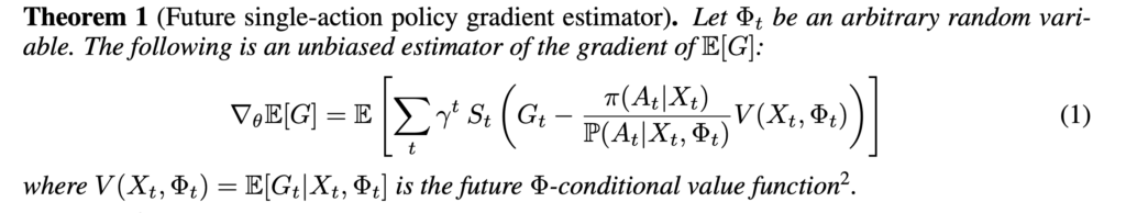
 contains the future part of the trajectory after time step
  . The intuition that in off-policy learning, we can utilize the steps after the current step to make better value estimation. However, I do not understand how
  represents.
 clusters with cluster centers
  . These cluster centers are trainable parameters. More importantly, these cluster centers will be used in every training batch. In each batch, we distort (augment) each image into two versions. For each version, the distorted images are transformed to an embedding space
 to be the image-cluster center similarity matrix, then the problem is converted to finding
  such that:

 data points. As illustrated in [1], they find the continuous code
  using the iterative Sinkhorn-Knopp algorithm.