I am reading Robert Nishihara’s thesis on Ray [1] while encountering several concepts I am not familiar with. So this post takes some notes on those new concepts.
Ring AllReduce
Ring AllReduce is a technique to communicate with multiple computation nodes for aggregating results. It is a primitive to many distributed training systems. In the Ray paper, the author tries to analyze how easy Ring AllReduce can be implemented using Ray’s API.
There are two articles that articulating the idea really well [5, 6]. They point out the bottleneck of network data communication when a distributed training system wants to aggregate gradients from worker nodes in a master-slave pattern. Because each worker (say, there are P-1 workers in total) needs to send its gradient vector (say it uses N space) to master and the master needs to aggregate and send the updated model vector (same size as the gradient vectors) back to each worker for the next iteration, the data transferring through the network would be as large as 2*(P-1)*N, which scales linearly with the number of workers.
Ring AllReduce have multiple cycles of data transferring among all workers (P workers since we don’t need one for the master). But each cycle only transfers a small amount of data in each cycle such that the accumulative amount of data transferring would be smaller than that of the master-slave pattern.
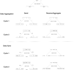
The basic idea of RingAllReduce is to divide each gradient vector into P chunks on all workers. There are first P-1 cycles of data aggregating then P-1 cycles data syncing. In the first cycle, each worker  sends its i-th chunk to the next worker (with index
  ), and receives the (i-1)-th chunk from the previous worker. The received (i-1)-th chunk will be aggregated locally with the worker’s own (i-1)-th chunk. In the second cycle, each worker sends its (i-1)-th chunk, which got aggregated in the last cycle, to the next worker, and receives (i-2)-th chunk from the previous worker. Similarly, each worker now can aggregate on its (i-2)-th chunk with the received chunk which also indexes on i-2. Continuing on this pattern, each worker will send its (i-2), (i-3)-th, …chunk in each cycle until
  data aggregating cycles are done. Upon then each worker has one chunk that has been fully aggregated with all other workers. Then doing the similar circular cycles P-1 times can make all workers sync on all fully aggregated chunks from each other.
I draw one simple diagram to illustrate the idea:
ADMM (Alternating Direction Method of Multipliers)
Another interesting technique introduced in the thesis is ADMM. It is a good opportunity to revisit optimization from the scratch. I’m mainly following [4] and [7] for basic concepts.
The definition of directional derivative and gradient:
The gradient of  is
is  . The gradient is a vector and can only be known fully when given a concrete value
  . The directional derivative is the gradient’s projection on another unit vector
  :
:  , where
  is inner product. See some introduction in [9] and [10].
The definition of a proper function simply means (Definition 51.5 [7]):  for all and
  for some .
The definition of a convex and strictly convex function is (Proposition 40.9 [7]):
The function  is convex on
  iff
iff  . Remember that
  is the change of
  caused by a tiny change in
  and we have
  . is a strict convex function iff
  .
.
This definition actually leads to a very common technique to check if a multivariate quadratic function is a convex function: if  , as long as
  is positive semidefinite, then is convex. See Example 40.1 [7].
The definition of affine hull: given a set of vectors  with
with  ,
,  is all affine combinations of the vectors in
  , i.e.,
  .
.
The definition of relint (Definition 51.9 [7]):
Suppose  a subset of
  , the relative interior of is the set:
  . There is a good example from [8] which explains the difference between interior and relative interior.
The most important thing is to understand the high level of the typical optimization procedure, which I also covered in [3]. Suppose we want to optimize the primal problem:
minimize 
subject to 

with 
The Lagrangian  for the primal problem is defined as:
 , where
  (i.e.,
  ) and
) and  .
.
The KKT conditions are necessary conditions that if  is a local minimum of , then must satisfy the following conditions [11]:
1. stationarity: 
2. primal feasibility:  and
and 
3. dual feasibility: 
4. complementary slackness: 
In other words, if we already know we know it must satisfy the KKT conditions. However not all solutions that satisfy the KKT conditions are the local minimum of . The KKT conditions can be used to find global minimum if additional conditions are satisfied. One such conditions is “Second-order sufficient conditions” [12], which I also talked about in [3]. Another such conditions are if the constraints, the domain  , and the objective function
  are convex, then KKT conditions also imply is a global minimum. (Theorem 50.6 [7]).
While some problems have characteristics that allow using the KKT conditions as sufficient condition to find the global solution, there are others that are easier to solve or approximate using another method called dual ascent. By maximizing another function called dual function, we can get the exact solution or a lower bound of the primal problem.
The dual function  is defined as:
The dual problem is defined as:
maximize 
subject to 
From [7] page 1697, one of the main advantages of the dual problem over the primal problem is that it is a convex optimization problem, since we wish to maximize a concave objective function  (thus minimize
  , a convex function), and the constraints
  are convex. In a number of practical situations, the dual function can indeed be computed.
If the maximum of the dual problem is  and the minimum of the primal problem is
  . We have weak duality that always holds:
  . Strong duality holds when the dual gap is zero, with certain conditions holding, for example slater’s condition [14]. We can find the local minimum
  of the dual problem by a special form of gradient ascent algorithm called sequential optimization problem (SMO) [13] because special treatment is needed for the constraints involved in the dual problem.
[7] provides two ways on how to do constrained optimization on SVM (Section 50.6 and 50.10): one is to use the KKT conditions, the other is to solve the dual problem.
The dual problem is simplified when there are only affine equality constraints in the primal problem:
Primal problem:
minimize 
subject to 
Dual problem:
maximize 
subject to 
Since the dual problem is an unconstrained optimization problem, we can use dual ascent to solve this problem easily:
 ,
,
where  is a step size.
The main flaw of the dual ascent is that under certain conditions the solution may diverge. The augmented Lagrangian method augments the Lagrangian function with a penalty term:
Based on some theory, the augmented Lagrangian is strongly convex and has better convergence property.
The method of multipliers is the dual ascent applied on the augmented Lagrangian:

If can be separated into two parts such that  , then we can iteratively update
  ,
,  , and
, and  separately, and such a method is called Alternating Direction Method of Multipliers (ADMM):
Primal problem:
minimize 
subject to 
The augmented Lagrangian:
Updates (note we are not doing  as in the method of multipliers):


If we define  and
and  , then the updates can be simplified as:


Structures in ,  , , and
  can often be exploited to carry out -minimization and -minimization more efficiently. We now look at several examples.
Example 1: if  is an identity matrix,
  , and
, and  is the indicator function of a closed nonempty convex set
  , then
  , which means
  is the projection of
  onto .
Example 2: if  and , then
  becomes an unconstrained quadratic programming with the analytic solution at
  .
.
Example 3: if  and it must satisfy
  , then the ADMM primal problem becomes:
minimize  (where
  is an indicator function of the nonnegative orthant
  )
)
subject to 
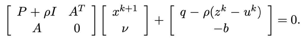
Then  . This is a constrained quadratic programming. We have to use KKT conditions to solve it. Suppose the Lagrangian multiplier is
  , then the KKT conditions state that:
 ,
,
which is exactly given by a linear system in matrix form in Section 5.2 [4]:
(As a side note, solving a constrained quadratic programming usually relies on KKT conditions. It can be converted to solving a linear system in matrix form: https://www.math.uh.edu/~rohop/fall_06/Chapter3.pdf)
Example 4 (Section 4.4.3 in [4]): if  , , and , then
  where is the soft thresholding operator.
References
[1] On Systems and Algorithms for Distributed Machine Learning: https://www2.eecs.berkeley.edu/Pubs/TechRpts/2019/EECS-2019-30.pdf
[2] Compare between parameter servers and ring allreduce: https://harvest.usask.ca/bitstream/handle/10388/12390/CHOWDHURY-THESIS-2019.pdf?sequence=1&isAllowed=y
[3] Overview of optimization: https://czxttkl.com/2016/02/22/optimization-overview/
[4] ADMM tutorial: https://web.stanford.edu/~boyd/papers/pdf/admm_distr_stats.pdf
[5] https://tech.preferred.jp/en/blog/technologies-behind-distributed-deep-learning-allreduce/
[7] Algebra, Topology, Differential Calculus, and Optimization Theory For Computer Science and Machine Learning https://www.cis.upenn.edu/~jean/math-deep.pdf
[8] https://math.stackexchange.com/a/2774285/235140
[10] https://math.stackexchange.com/a/661220/235140
[11] https://en.wikipedia.org/wiki/Karush%E2%80%93Kuhn%E2%80%93Tucker_conditions#Necessary_conditions
[12] https://en.wikipedia.org/wiki/Karush%E2%80%93Kuhn%E2%80%93Tucker_conditions#Sufficient_conditions