Constrained RL / Multi-Objective RL

Learning a policy that can optimize multiple types of rewards or satisfy different constraints is a much desired feature in the industry. In real products, we often care about not only single one metric but several that interplay with each other. For example, we want to derive a policy to recommend news feeds which expects to increase impressions but should not regress the number of likes, follows, and comments.

The vein of multi-objective and constrained RL is an active research area. Before we proceed, I want to clarify the definition of multi-objective RL and constrained RL in my own words. Multi-objective RL focuses on optimizing multiple objectives in the same time. For one reward type, the question is how we can maximize this reward type without reducing any of other rewards. Therefore, multi-objective RL usually needs to fit the whole Pareto Frontier. Constrained RL is somewhat relaxed because its focused question is how we can maximize this reward type while other rewards are no worse than specified constraints (which don’t need to be “not reduce any of other rewards).

Multi-Objective RL

Constrained RL

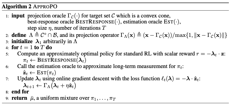
[1] introduces an algorithm called ApproPO to answer the feasibility problem and return the best policy if the problem is feasible. The feasibility problem is defined as:

$\text{Find } \mu \in \triangle{(\Pi)} \text{ such that } \bar{\pmb{z}}(\mu) \in \mathcal{C},$

which can be expressed as a distance objective:

$\min\limits_{\mu \in \triangle(\Pi)} dist(\bar{\pmb{z}}(\mu), \mathcal{C})$

Here, $\triangle(\Pi)$ denotes all possible mixed policies so you should think $\mu$ as a probability distribution over finitely many stationary policies. $\bar{\pmb{z}}(\cdot) \in \mathbb{R}^d$ is a $d$ -dimensional return measurement vector (i.e., $d$ is the number of rewards over which we specify constraints). $\bar{\pmb{z}}(\mu)$ could then be thought as a weighted sum of returns of individual stationary policies: $\bar{\pmb{z}}(\mu)=\sum\limits_{\pi} \mu(\pi)\bar{\pmb{z}}(\pi)$ . $C$ is the convex set of constraints. Why couldn’t we just get one single stationary policy as the answer? It seems to me that ApproPO has to return a mixture of policies because the author chooses to solve the minimization problem by solving a two-player game based on game theory, which suggests “the average of their plays converges to the solution of the game”.

Here is the stretch of how the authors solve the minimization problem by solving a two-player game.

For a convex cone $\mathcal{C} \in \mathbb{R}^d$ and any point $\pmb{x} \in \mathbb{R}^d$ , we define the dual convex cone $\mathcal{C}^\circ \triangleq \{\pmb{\lambda}: \pmb{\lambda}\cdot \pmb{x} \leq 0 \text{ for all } \pmb{x}\in \mathcal{C}\}$ .
According to Lemma 3.2, $dist(\pmb{x}, \mathcal{C}) = \max\limits_{\pmb{\lambda} \in \mathcal{C}^\circ \cap \mathcal{B}} \pmb{\lambda} \cdot \pmb{x}$ . Plugging this Lemma into the minimization problem we actually care about, we obtain a min-max game (with $\pmb{x}=\bar{\pmb{z}}(\mu)$ ): $\min\limits_{\mu \in \triangle(\Pi)} \max\limits_{\pmb{\lambda} \in \mathcal{C}^\circ \cap \mathcal{B}} \pmb{\lambda} \cdot \bar{z}(\mu)$ .
The min-max formula satisfies certain conditions (as shown in the paragraph above Eqn. (9) in the paper [1]) such that it is equivalent to a max-min game: $\min\limits_{\mu \in \triangle(\Pi)} \max\limits_{\pmb{\lambda} \in \mathcal{C}^\circ \cap \mathcal{B}} \pmb{\lambda} \cdot \bar{\pmb{z}}(\mu) = \max\limits_{\pmb{\lambda} \in \mathcal{C}^\circ \cap \mathcal{B}} \min\limits_{\mu \in \triangle(\Pi)} \pmb{\lambda} \cdot \bar{\pmb{z}}(\mu)$ .
In the max-min game, the $\pmb{\lambda}$ -player plays first, and the $\mu$ -player plays next. And their turns can continue incessantly. Theory has shown that if the $\pmb{\lambda}$ -player keeps using a no-regret algorithm repeatedly against $\mu$ -player who uses a best response algorithm, then “the averages of their plays converge to the solution of the game”.
There is an off-the-shelf no-regret algorithm called online gradient descent (OGD) which can be used by $\pmb{\lambda}$ -player. We won’t cover the details of this algorithm in this post. Given any $\pmb{\lambda}$ returned by $\pmb{\lambda}$ palyer, the best response algorithm used by $\mu$ -player will need to find $\mu$ such that $\pmb{\lambda} \cdot \bar{\pmb{z}}(\mu)= \sum\limits_{\pi}\mu(\pi) \cdot (\pmb{\lambda}\cdot\bar{\pmb{z}}(\pi))$ is minimized. The implicit conditions that the best response algorithm’s solution should also satisfy are $\sum\limits_\pi u(\pi)=1$ and $0 \leq u(\pi) \leq 1$ for $\forall \pi$ .
Based on properties of linear programming, we know the best response algorithm’s solution must be on a corner point. This can be translated into finding a single stationary policy $\pi$ which optimizes the return with the scalar reward $-\pmb{\lambda}\cdot \bar{\pmb{z}}$ . Such a $\pi$ will be found using any preferred RL algorithm on the MDP.
After $\mu$ -player returns the best $\mu$ , $\lambda$ -player can again return a new $\pmb{\lambda}$ based on $\bar{\pmb{z}}(\mu)$ . Then $\mu$ -player again returns the best policy learned on the scalar reward $-\pmb{\lambda}\cdot \bar{\pmb{z}}$ . The iterations go on for $T$ steps. Finally the algorithm would return a random mixture of $\mu$ from all iteration steps.

My concern is that this algorithm could not easily be extended to the batch learning context. Although the best response algorithm can always use an off-policy algorithm to learn $\pi$ without recollecting data, determining the optimal $\pmb{\lambda}$ needs to know $\bar{\pmb{z}}(\pi)$ , the estimation of $\pi$ on all dimensions of rewards. This would be super inaccurate using any off-policy evaluation method. There is also a question on how to serve the mixture of policies rather than just one single policy.

References

[1] Reinforcement Learning with Convex Constraints

Constrained RL / Multi-Objective RL

Leave a comment

Cancel reply