Notes on “Soft Actor-Critic: Off-Policy Maximum Entropy Deep Reinforcement Learning with a Stochastic Actor”

I am reading this paper (https://arxiv.org/abs/1801.01290) and wanted to take down some notes about it.

Introduction

Soft Actor-Critic is a special version of Actor-Critic algorithms. Actor-Critic algorithms are one kind of policy gradient methods. Policy gradient methods are different than value-based methods (like Q-learning), where you learn Q-values and then infer the best action to take at each state $s$ using $\arg\max_a Q(s,a)$ . Policy gradient methods do not depend on value functions to infer the best policy, instead they directly learn a probability function $\pi(a|s)$ . However policy gradient methods may still learn value functions for the purpose of better guiding the learning of the policy probability function $\pi(a|s)$ .

We have introduced several kinds of policy gradient methods in [2, 18]. Here, we briefly recap. The objective function of policy gradient methods is:

$J(\theta)=\mathbb{E}_{s,a\sim\pi}Q^{\pi}(s,a)$ ,
where $\theta$ is the parameter of the policy $\pi$ .

In problems with a discrete action space, we can rewrite the expectation in summation:

$J(\theta)=\mathbb{E}_{s,a\sim\pi}Q^{\pi}(s,a)=\sum\limits_{s \in S} d^\pi(s) V^\pi(s)=\sum\limits_{s \in S} d^\pi(s) \sum\limits_{a \in A} \pi(a|s) Q^\pi(s,a),$

where $d^\pi(s)$ is the stationary distribution of Markov chain for $\pi$ , $V^\pi(s)=\mathbb{E}_{a \sim \pi}[G_t|S_t=s]$ , and $Q^{\pi}(s,a)=\mathbb{E}_{a \sim \pi}[G_t|S_t=s, A_t=a]$ . $G_t$ is accumulated rewards since time step $t$ : $G_t=\sum^\infty_{k=0}\gamma^k R_{t+k}$ .

Policy gradient methods strive to learn the values of $\theta$ , which is achieved through gradient ascent w.r.t. $J(\theta)$ . The gradient $\nabla_\theta J(\theta)$ is obtained by the policy gradient theorem (proved in [4]):

$\nabla_\theta J(\theta) = \mathbb{E}_{s,a\sim\pi}[Q^\pi(s,a)\nabla_\theta log \pi_\theta(a|s)]$

Different policy gradient methods use different methods to estimate $Q^\pi(s,a)$ : REINFORCE uses a Monte Carlo method in which empirical accumulated rewards $G_t$ is used to unbiasedly approximate $Q^\pi(s,a)$ ; state-value actor-critic learns a value function $V_w(s)$ and uses $R+\gamma V_w(s')$ to approximate $Q^\pi(s,a)$ ; action-value actor-critic learns a Q-value function $Q_w(s,a)$ and uses $R+\gamma Q_w(s',a')$ to approximate $Q^\pi(s,a)$ . Note that since $\nabla_\theta J(\theta)$ is in an expectation form $\mathbb{E}_{s,a \sim \pi} [\cdot]$ , we need to collect on-policy samples. That’s why the soft actor-critic papers mentions in Introduction:

“some of the most commonly used deep RL algorithms, such as TRPO, PPO, A3C, require new samples to be collected for each gradient step.”

If we have only off-policy samples instead, which are collected by $\pi_b$ , $J(\theta)$ becomes “the value function of the target policy, averaged over the state distribution of the behavior policy” (from DPG paper [19]):

$J(\theta)=\mathbb{E}_{s\sim \pi_b} \left[ \mathbb{E}_{a\sim\pi}Q^{\pi}(s,a) \right]$

The critical problem presented by this formula is that if you take derivative of $J(\theta)$ w.r.t. $\theta$ , you’d better to be able to write the gradient without $\mathbb{E}_{a\sim\pi}[\cdot]$ because any such gradient can’t be computed using mini-batches collected from $\pi_b$ . Rather, we have several choices to learn $\theta$ given this off-policy objective $J(\theta)$ :

Using importance sampling, rewrite $\mathbb{E}_{a\sim\pi}\left[ Q^{\pi}(s,a)\right]$ as $\mathbb{E}_{a\sim\pi_b}\left[\frac{\pi(a|s)}{\pi_b(a|s)}Q^{\pi_b}(s,a) \right]$ . This results to the gradient update $\mathbb{E}_{s,a \sim \pi_b} [\frac{\pi(a|s)}{\pi_b(a|s)} Q^{\pi_b}(s,a) \nabla_\theta log \pi(a|s)]$ . See [18]. However, importance sampling can cause great variance empirically.
Making the policy deterministic would remove the expectation $\mathbb{E}_{a\sim\pi}[\cdot]$ . $J(\theta)$ then becomes $J(\theta)=\mathbb{E}_{s\sim\pi_b}\left[Q^{\pi}(s,\pi(s))\right]$ . The gradient update can be computed as $\mathbb{E}_{s\sim \pi_b}\left[ \nabla_\theta \pi(s) \nabla_a Q^\pi(s,a)|_{a=\pi(s)}\right]$ . This is how DPG works. See [20].
Using reparametrization trick (covered more below), which makes $\pi(a|s) = \pi^{deterministic}(s)+\epsilon$ , a deterministic function plus an independent noise, we would have $J(\theta)=\mathbb{E}_{s\sim\pi_b, \epsilon \sim p_\epsilon}\left[Q^{\pi}(s,\pi(s))\right]$ . The gradient update would be: $\mathbb{E}_{s\sim\pi_b, \epsilon \sim p_\epsilon}\left[\nabla_a Q^{\pi}(s,a)|_{a=\pi(s)} \nabla_\theta \pi(s) \right] \newline=\mathbb{E}_{s\sim\pi_b, \epsilon \sim p_\epsilon}\left[\nabla_a Q^{\pi}(s,a)|_{a=\pi(s) } \nabla_\theta \pi^{deterministic}(s) \right]$

The third method is used in Soft Actor-Critic, although SAC adds some more ingredients. Let’s now dive into it.

Soft Actor-Critic

Soft Actor-Critic (SAC) is designed to be an off-policy policy-gradient method. What makes it special is that it strives to maximize long-term rewards as well as action randomness, because more random actions mean better exploration and robustness. Therefore, in the maximum entropy framework, the objective function can be formulated as:

$J(\pi)=\sum\limits^T_{t=0}\mathbb{E}_{(s_t, a_t)\sim\rho_\pi} \left[r(s_t, a_t) + \alpha \mathcal{H} \left( \pi\left(\cdot | s_t \right) \right) \right],$

where $\mathcal{H}(\pi( \cdot | s ) )$ of an action distribution $\pi(\cdot|s)$ is the entropy defined as $\mathbb{E}_{a \sim \pi(\cdot|s_t)}[-log \pi(a|s)]$ , and $\alpha$ is the term controlling the influence of the entropy term.

We can always treat $\alpha=1$ by subsuming it into the reward function. Therefore, with $\alpha$ omitted, we have the following objective function, soft Q-function update operator, and soft value function:

(1) $J(\pi)=\sum\limits^T_{t=0}\mathbb{E}_{(s_t, a_t)\sim\rho_\pi} \left[r(s_t, a_t) + \mathcal{H} \left( \pi\left(\cdot | s_t \right) \right) \right]$

(2) $\mathcal{T}^\pi Q(s_t, a_t) \triangleq r(s_t, a_t) + \gamma \mathbb{E}_{s_{t+1}\sim p}\left[V(s_{t+1})\right]$

(3) $V(s_t) = \mathbb{E}_{a_t \sim \pi}\left[Q(s_t, a_t) - \log \pi(a_t|s_t) \right]$

Derivation

The paper uses Lemma1, Lemma 2 and Theorem 1 to prove the learning pattern will result in the optimal policy that maximizes the objective in Eqn. (1). The tl; dr is that Lemma1 proves that soft Q-values of any policy would converge rather than blowing up; Lemma2 proves that based on a policy’s soft Q-values, you can find a no-worse policy.

Lemma 1 proof

Screen Shot 2018-11-09 at 12.05.04 PM

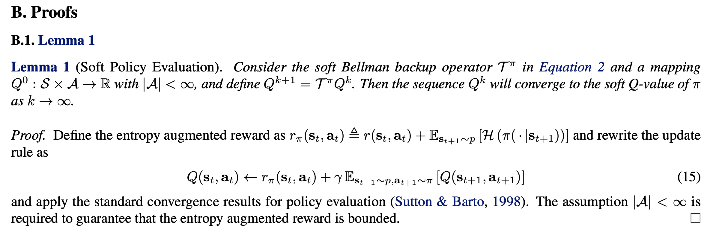
“The standard convergence results for policy evaluation” means:

(1) there exists a fixed point $Q^\pi$ because of the way we define Eqn.15: for each state $s$ and each action $a$ , we define one equation of Eqn.15. We have $|S|+|A|$ equations in total. And there are $|S|+|A|$ dimensions of $Q^\pi$ . Therefore, there exists a unique fixed point: $Q^\pi=r+\gamma P^\pi Q^\pi$ , where $P^\pi$ is the operator for calculating expectation $\mathbb{E}[\cdot]$ .

(2) prove $T^\pi$ is a $\gamma$ -contraction under the infinity norm, i.e., $\Vert T^\pi Q^{k+1} - T^\pi Q^k \Vert_\infty \leq \gamma \Vert Q^{k+1} - Q^{k}\Vert_\infty$ . Explained in plain English, $T^\pi$ being a $\gamma$ -contraction means consecutive application of $T^\pi$ make the function $Q$ closer to the fixed point $Q^\pi$ at the rate of $\gamma$ .

The proof is found from [6]:

$\Vert T^\pi Q^{k+1} - T^\pi Q^k \Vert_\infty \newline =\Vert r +\gamma P^\pi Q^{k+1} - r - \gamma P^\pi Q^{k} \Vert_\infty \newline =\gamma \Vert P^\pi(Q^{k+1}-Q^k) \Vert_\infty \newline \leq \gamma \Vert Q^{k+1}-Q^k \Vert_\infty$

The last two steps are derived using $\Vert Tx\Vert_\infty \leq \Vert T \Vert_\infty \Vert x \Vert_\infty$ from [7] and the fact that $\Vert P^\pi \Vert_\infty = 1$ (because $P^\pi$ is the operator for $\mathbb{E}[\cdot]$ , though I have not verified this fact though).

(3) therefore, by contraction theory (Theorem 5.1-2 in [10]), applying $T^\pi$ will eventually lead to $Q^\pi$ . [9]

Convergence of policy evaluation/value evaluation usually have the similar pattern, such as the one for Q-learning [8].

Lemma 2 proof

Screen Shot 2018-11-09 at 3.39.57 PM

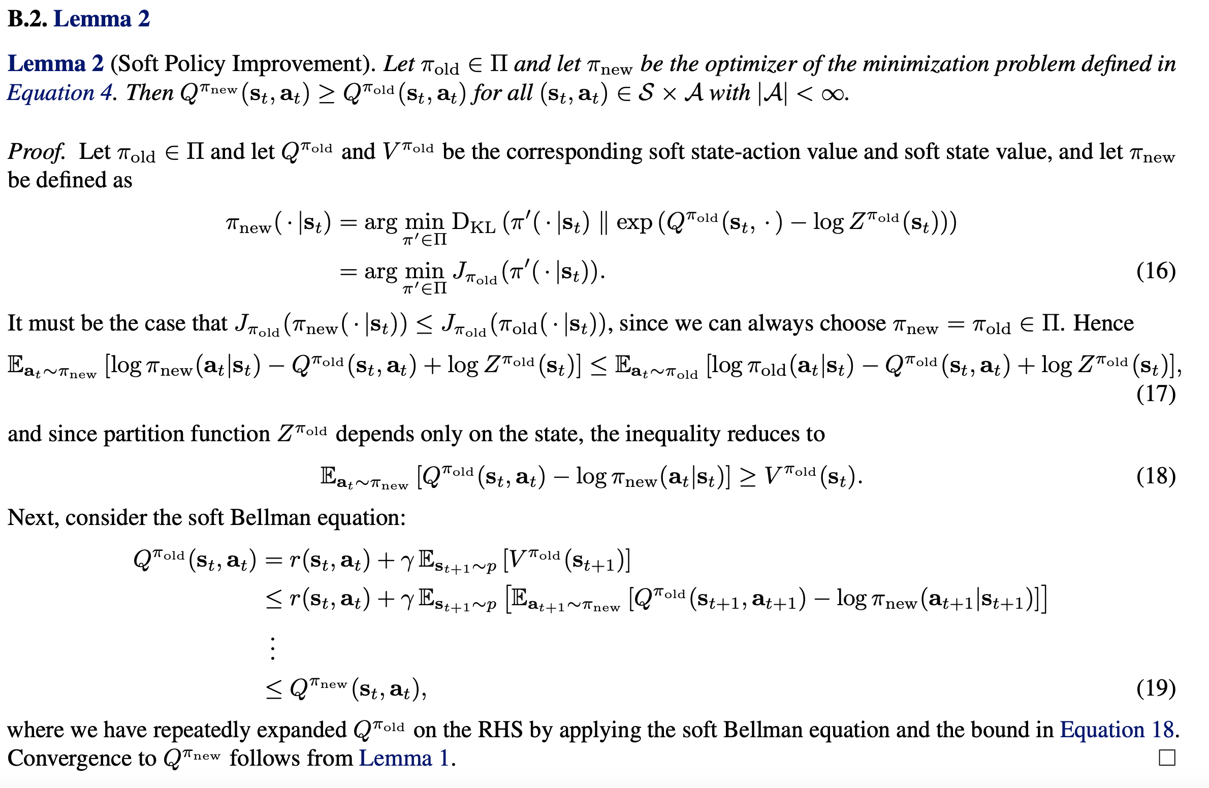
Proving Lemma 2 is basically just expanding $KL$ -divergence formula $D_{KL}(P|Q)=\int^{\infty}_{-\infty}p(x)\frac{p(x)}{q(x)}dx$ . From Eqn. 16, we expand $KL$ -divergence formula as:

$J_{\pi_{old}}(\pi'(\cdot|s_t)) \newline \triangleq D_{KL} (\pi'(\cdot | s_t) \; \Vert \; exp(Q^{\pi_{old}}(s_t, \cdot) - \log Z^{\pi_{old}}(s_t)) ) \newline = - \int \pi'(a_t | s_t) \log \frac{exp(Q^{\pi_{old}}(s_t, a_t) - \log Z^{\pi_{old}}(s_t)))}{\pi'(a_t|s_t)} d a_t \newline = \int \pi'(a_t | s_t) \big(\log \pi'(a_t|s_t) + \log Z^{\pi_{old}}(s_t) - Q^{\pi_{old}}(s_t, a_t) ) \big) d a_t \newline = \mathbb{E}_{a_t \sim \pi'}[\log \pi'(a_t|s_t) + \log Z^{\pi_{old}}(s_t) - Q^{\pi_{old}}(s_t, a_t) )]$

Note that the authors defined a new objective function $J_{\pi_{old}}(\pi'(\cdot|s_t))\triangleq D_{KL} (\pi'(\cdot | s_t) \; \Vert \; exp(Q^{\pi_{old}}(s_t, \cdot) - \log Z^{\pi_{old}}(s_t)) )$ , which is different than Eqn.1. The purpose of defining $J_{\pi_{old}}(\pi'(\cdot|s_t))$ is to help us get to Eqn. 18, which is then used to prove $Q^{\pi_{old}}(s_t, a_t) \leq Q^{\pi_{new}}(s_t, a_t)$ in Eqn. 19.

Implementation

Since we are looking at cases with continuous actions, the authors suppose we use a network to output mean and standard deviation for a (multi-dimensional) Gaussian. In other words, this network has an output vector for action means $\mu$ , and another output vector for action standard deviations $\sigma$ . The action that is to be taken will be sampled from $\mathcal{N}(\mu, \sigma^2)$ .

export

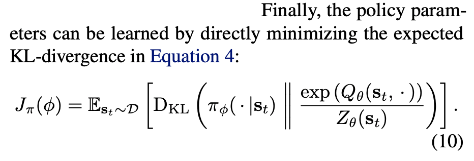
Since $D_{KL}(p\Vert q) = \mathbb{E}_{x \sim p(x)}[\log p(x) - \log q(x)]$ , $J_\pi(\phi)$ can be rewritten as:

$J_\pi(\phi) = \mathbb{E}_{s_t \sim \mathcal{D}, a_t \sim \pi_\phi}[\log \pi_\phi(a_t | s_t) - Q_\theta(s_t, a_t)]$

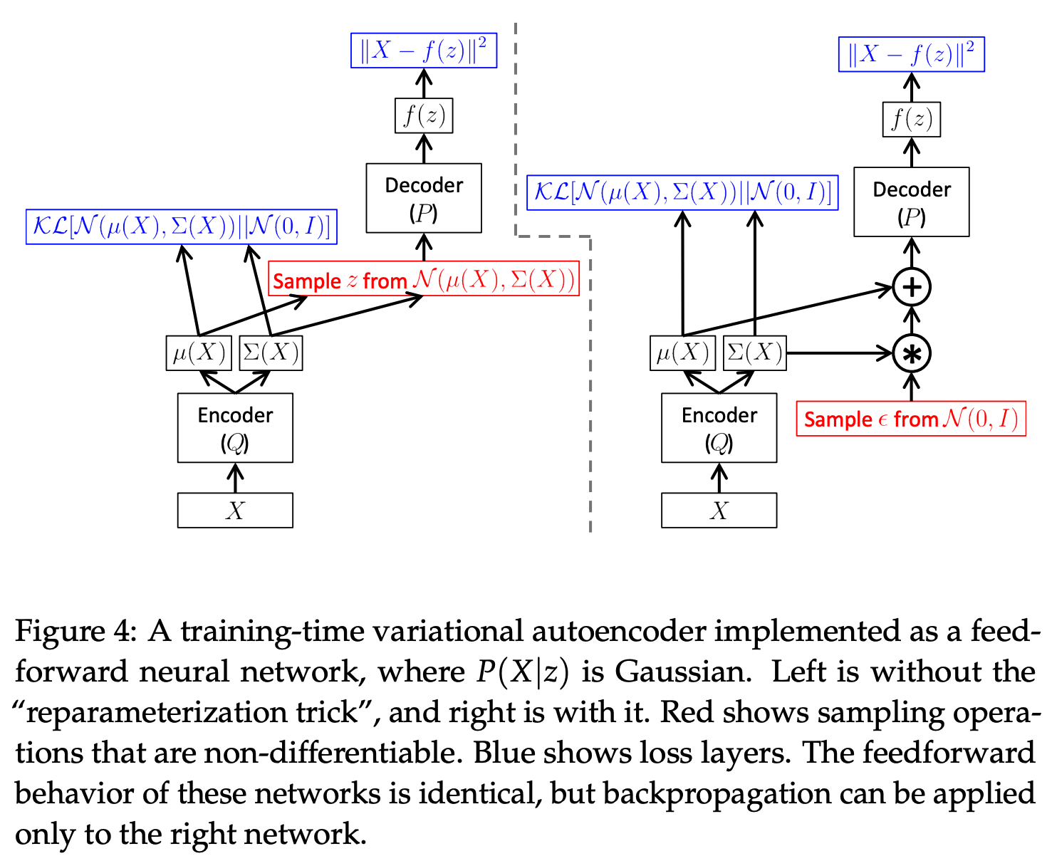
However, actions are sampled from the policy network’s output, which are represented as a stochastic node in the computation graph. Gradient cannot be backprogagated unless we use “reparameterization trick” to make the action node a deterministic node. In other word, actions will be outputted from a deterministic function $f(\cdot |s_t)$ with a stochastic input $\epsilon_t$ . This trick is also widely used in variational autoencoders, and has been discussed in [11, 13, 14, 15, 16] . Reparameterization trick can also be illustrated in the diagram below [11]:

Screen Shot 2018-11-11 at 7.17.57 PM

After applying reparameterization trick, we have the stochastic gradient, for a training tuple $(s_t, a_t)$ :

$\hat{\nabla}_\phi J_\pi(\phi) \newline = \nabla_\phi [\log \pi_\phi(a_t | s_t) - Q_\theta(s_t, a_t)] |_{a_t = f_\phi(\epsilon_t ; s_t)} \newline = (\nabla_{a_t} \log \pi_\phi(a_t | s_t) - \nabla_{a_t} Q_\theta (s_t, a_t)) \nabla_\phi f_\phi(\epsilon_t; s_t)$

I think what I derived above is a little different than Eqn.(13) in the paper, which has an extra $\nabla_\phi \log \pi_\phi(a_t|s_t)$ . Right now I am not sure why but I will keep figuring it out.

In applications where output actions need to be squashed to fit into some ranges, $\pi_\phi(|s_t)$ also needs to account that. Basically, if squashed action = squash function(raw_action), then the probability density of squashed actions will be different than the probability density for raw actions [17]. The original code reflects this in https://github.com/haarnoja/sac/blob/fba571f81f961028f598b0385d80cb286d918776/sac/policies/gaussian_policy.py#L70-L75.

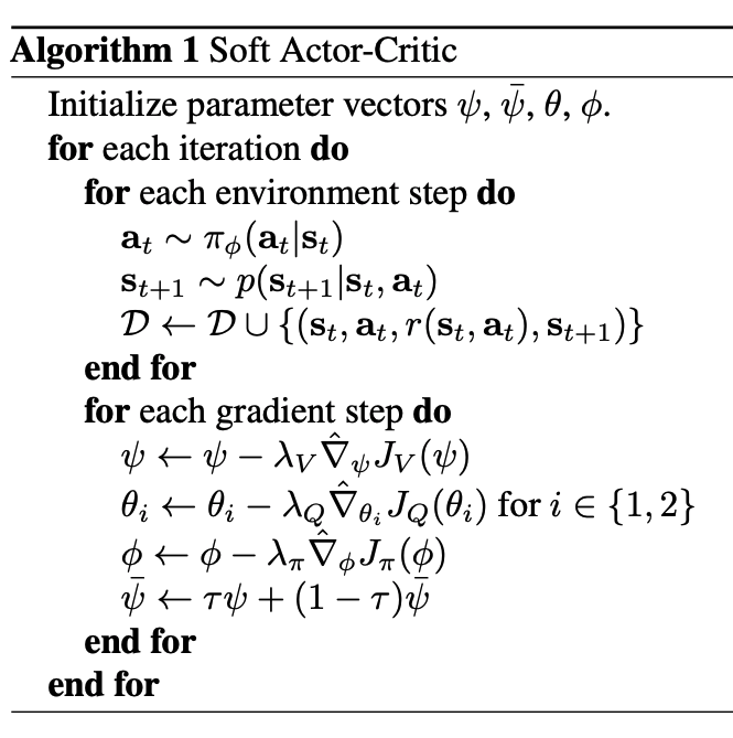
SAC’s learning pattern is summarized as follows:

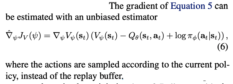
It evaluates the soft Q-value function and the soft value function. Both functions are associated with the train policy but can still be learned through the data collected by the behavior policy.

To estimate the soft value function, we can draw states from experience replay generated by the behavior policy, and use the action generated by the train policy.

Screen Shot 2019-01-31 at 3.34.46 PM

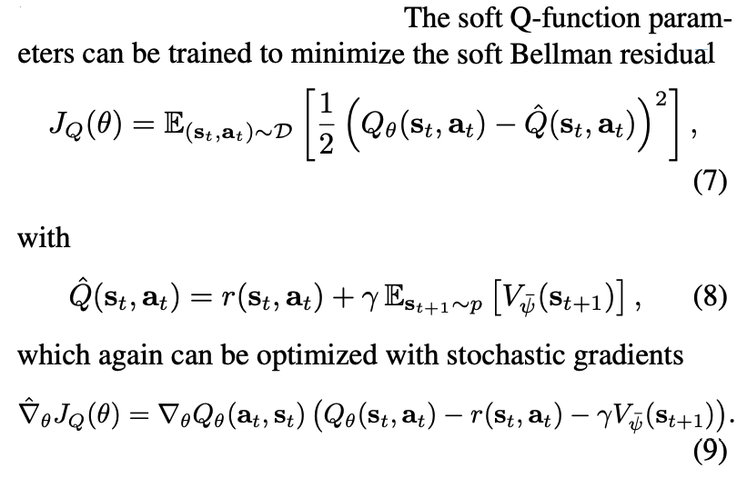
To estimate the Q-value function, we can just use states and actions both drawn from the experience replay:

Screen Shot 2019-01-31 at 3.38.09 PM

2. It updates the policy parameters, with the goal to minimize the expected KL-divergence between the current policy outputs and the exponential of the soft Q-value function.

3. Loop back to step 1

Thee pseudocode is as follows:

Screen Shot 2019-01-31 at 2.15.35 PM

Lastly, I am using the slides for soft actor-critic paper to end this post [12].

References

[1] Mnih, V., Badia, A. P., Mirza, M., Graves, A., Lillicrap, T., Harley, T., … & Kavukcuoglu, K. (2016, June). Asynchronous methods for deep reinforcement learning. In International conference on machine learning (pp. 1928-1937). https://arxiv.org/pdf/1602.01783.pdf

[2] Policy gradient: https://czxttkl.com/?p=2812

[3] Differences between on-policy and off-policy: https://czxttkl.com/?p=1850

[4] https://lilianweng.github.io/lil-log/2018/04/08/policy-gradient-algorithms.html#soft-actor-critic

[5] Off-Policy Actor-Critic: https://arxiv.org/abs/1205.4839

[6] http://mlg.eng.cam.ac.uk/teaching/mlsalt7/1516/lect0304.pdf

[7] https://czxttkl.com/?p=2616

[8] http://users.isr.ist.utl.pt/~mtjspaan/readingGroup/ProofQlearning.pdf

[9] https://www.cs.cmu.edu/~katef/DeepRLControlCourse/lectures/lecture3_mdp_planning.pdf

[10] Kreyszig, E. (1978). Introductory functional analysis with applications (Vol. 1). New York: wiley.

[11] Tutorial on Variational Autoencoders

[12] slides for soft actor-critic

[13] https://stats.stackexchange.com/questions/199605/how-does-the-reparameterization-trick-for-vaes-work-and-why-is-it-important

[14] Reparameterization Trick Notebook

[15] The Reparameterization “Trick” As Simple as Possible in TensorFlow

[16] arxiv insight: variational autoencoders

[17] Change of variable in probability density

[18] https://czxttkl.com/2020/02/18/practical-considerations-of-off-policy-policy-gradient/

[19] http://proceedings.mlr.press/v32/silver14.pdf

[20] https://czxttkl.com/2019/01/10/dpg-and-ddpg/

Join the Conversation

1 Comment

Ben You says:

May 1, 2023 at 10:05 pm

“I think what I derived above is a little different than Eqn.(13) in the paper, which has an extra \nabla_\phi \log \pi_\phi(a_t|s_t). Right now I am not sure why but I will keep figuring it out.”

The missing item is due to the following reason:
The gradient operator should be moved inside the expectation (not directly interchange) before the sampling.

Please refer to https://medium.com/@amiryazdanbakhsh/gradients-of-the-policy-loss-in-soft-actor-critic-sac-452030f7577d