Reinforcement learning algorithms can be divided into many families. In model-free temporal difference methods like Q-learning/SARSA, we try to learn action value  for any state-action pair, either by recording (“memorizing”) exact values in a tabular or learning a function to approximate it. Under
  -greedy, the action to be selected at a state will therefore be
  but there is also a small constant chance to be any non-optimal action.
Another family is called policy gradient methods which directly map states to actions. To select actions, they do not need to consult a value table or a value function. Instead, each action can be selected with a probability determined by a parameterized policy function  , where
  is the policy function’s parameters.
The advantages of policy gradient methods over Q-learning/SARSA using greedy are mainly two:
- in some situations the optimal approximate policy must be stochastic. An example from [1]: in card games with imperfect information the optimal play is often to do two different things with specific probabilities, such as when bluffing in Poker. Action-value methods have no natural way of finding stochastic optimal policies.
- problems vary in the complexity of their policies and action-value functions. In some problems, the policy is a much simpler function to approximate than action-values so it will be faster to learn
The general update form of policy gradient methods is  , where
  is performance measure with respect to the policy weights.
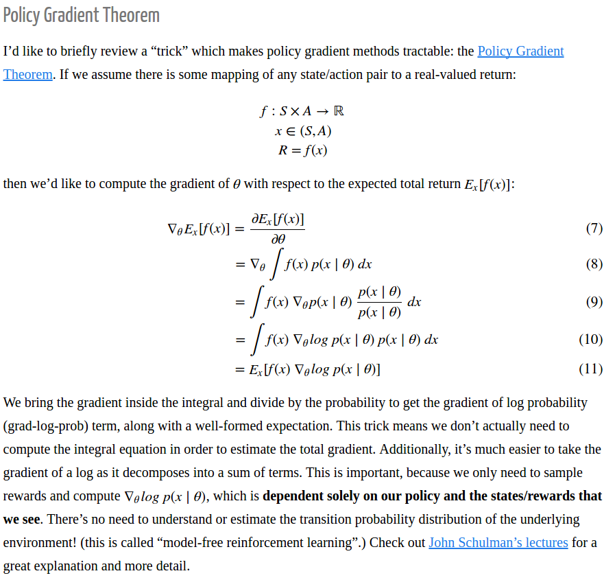
Now, the policy gradient theorem can be briefly described as [5]:
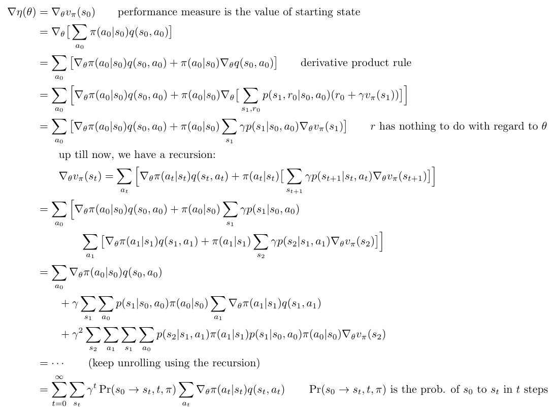
In episodic case, the policy gradient theorem derives as follows (according to [1]):
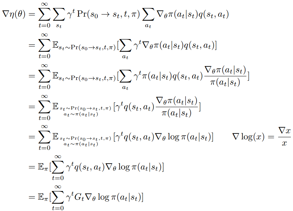
The last expression is an exact formula of the gradient of  . It can also be seen as an expectation of
  over the probability distribution of landing on
  in
in  steps. Please note for any fixed ,
  . Therefore, we can rewrite the above last expression as an expectation form:
where  .
.  is an unbiased estimator of
  in the last two steps since we do not have estimation for . We use
  to replace
  , meaning that the sequence
  are generated following the policy
  and the transition probability
  . Sometimes we can also write
  because the policy
  is parameterized by . We can also write as
  . In other words,
 ![\nabla \eta(\theta) = \mathbb{E}_{s_{0:T}, a_{0:T}}[\sum\limits_{t=0}^T \gamma^t G_t \nabla_\theta \log \pi(a_t|s_t)] &s=2](https://czxttkl.com/wp-content/ql-cache/quicklatex.com-093ef803c0ca0df70cae9b9ecec84de5_l3.png "Rendered by QuickLaTeX.com")
What we do in reality is to use these collected state, actions and rewards as samples to approximate the exact expectation of  :
:
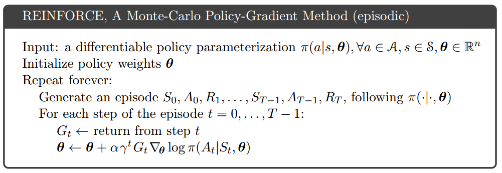
This kind of policy gradient method is called REINFORCE, by Ronald J. Williams from Northeastern University. The original paper [2] is hard to read in my opinion. It directly tells you what is the update rule of by construction, and then tells you the expected update aligns in the same direction as the performance gradient. What I wish to be told is how he derived the update rule of in the first place.
(Updated 09/18/2017: The same derivative procedure of REINFORCE is illustrated more clearly in [10])
(Updated 01/31/2020: The derivative procedure of REINFORCE in continuous state/action space is illustrated in [15])
One important extension of REINFORCE is to offsetting by a baseline  , a function of . Intuitively, we need not how good an action is, but how much better this action is compared to average actions. For example, if is uniformly larger than zero for either good or bad actions, will always get updated to encourage either kind of actions. We need to calibrate such that it can differentiate good or bad actions better. Mathematically, adding a baseline can reduce the variance of while still keeping it as unbiased estimator.
First, let’s look at why offsetting by still makes an unbiased estimator (reference from [8]):
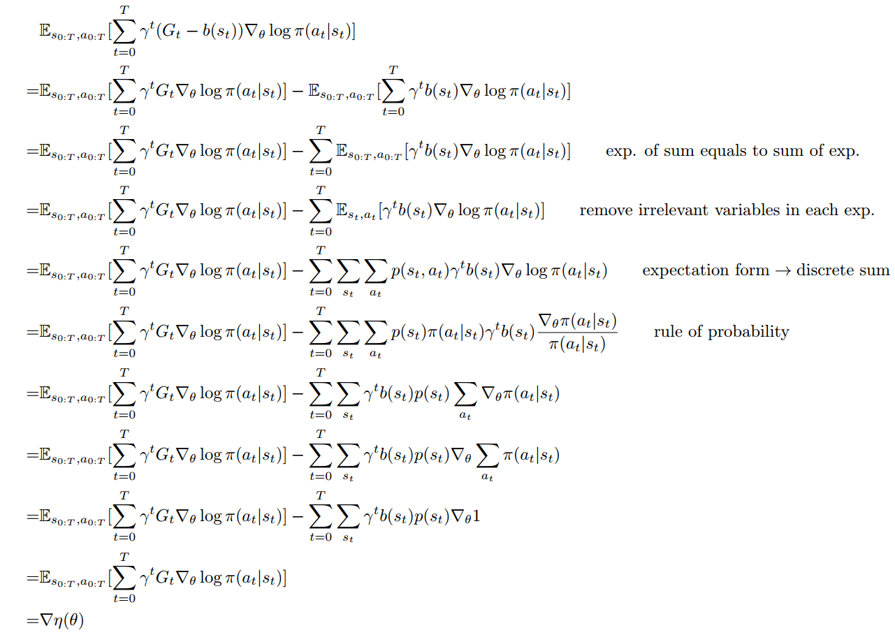
To ensure ![\mathbb{E}_{s_{0:T}, a_{0:T}} [\sum\limits_{t=0}^T \gamma^t (G_t - b(s_t)) \nabla_\theta \log \pi (a_t|s_t)]](https://czxttkl.com/wp-content/ql-cache/quicklatex.com-8d586d2f867e3a9f19be27fbca1afe2b_l3.png "Rendered by QuickLaTeX.com") is an unbiased estimate of , should only be a function of , but not
is an unbiased estimate of , should only be a function of , but not  . Otherwise
 ![\mathbb{E}_{s_{0:T}, a_{0:T}}[\sum\limits_{t=0}^T \gamma^t b(s_t) \nabla_\theta \log \pi (a_t | s_t)]](https://czxttkl.com/wp-content/ql-cache/quicklatex.com-39cb9ee96a8a70267a3c0f0de4ba410e_l3.png "Rendered by QuickLaTeX.com") is not zero.
is not zero.
It is less obvious that adding can reduce the variance of ![Var[ \sum\limits_{t=0}^T \gamma^t G_t \nabla_\theta \log \pi(a_t | s_t)]](https://czxttkl.com/wp-content/ql-cache/quicklatex.com-00b7d15eb73cf2b088fdad5a69ff16ac_l3.png "Rendered by QuickLaTeX.com") .
.
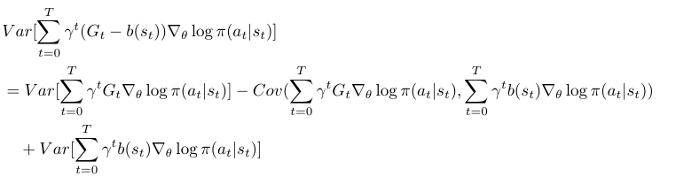
From here, we can see if  has large enough covariance with
  to outweigh its own variance, then the variance is reduced. Unrealistically, if
  , then variance will be zero, although this is impossible because is only a function of without magic forecast ability to 100% approach .
(sidenote: I cannot follow [8]’s deduction on variance reduction part.)
One way is to train a predictor on  with parameter
  as a baseline:
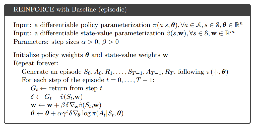
From [1]: Note that REINFORCE uses the complete return from time t (), which includes all future rewards up until the end of the episode. In this sense REINFORCE is a Monte Carlo algorithm and is well defined only for the episodic case with all updates made in retrospect after the episode is completed.
When we derived , we use the property that ![\mathbb{E}[G_t|S_t, A_t]=q_\pi(s_t, a_t)](https://czxttkl.com/wp-content/ql-cache/quicklatex.com-d172bdd4b1e22f48ae494f1aa7a44c42_l3.png "Rendered by QuickLaTeX.com") . However, could have high variance because it involves returns from step to
. However, could have high variance because it involves returns from step to  , where each reward can be seen as a random variable [13]. An alternative estimator of
  which has lower variance but higher bias is to use “bootstrapping”, i.e., use a parameterized value function
  plus the next immediate reward to approximate
  . The one-step actor-critic algorithm is described as follows [1]:
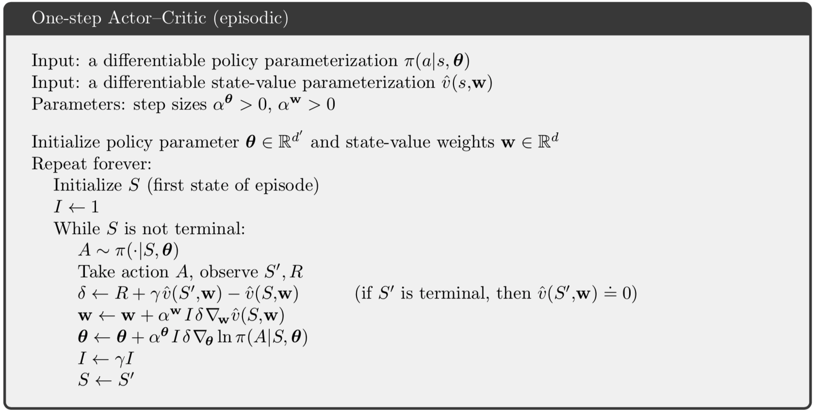
REINFORCE is an on-policy algorithm because  in the gradient update depends on , the returns generated by following the current policy
  . The specific one-step actor-critic algorithm we just described is also an on-policy algorithm because
  depends on the next state
  which is the result of applying at the current state
  . There also exists off-policy actor-critics, see an overview of on-policy and off-policy policy gradient methods at [14].
A more recent advance in baseline is Generalized Advantage Estimation (GAE) [6]. They introduce two parameters,  and
and  , in an un-discounted reward problem to help estimate
 ![g:=\nabla_\theta \mathbb{E}[\sum_{t=0}^\infty] r_t](https://czxttkl.com/wp-content/ql-cache/quicklatex.com-675a43e0384f3db1622065126706063a_l3.png "Rendered by QuickLaTeX.com") with little introduced bias and reduced variance. (Note that how discounted reward problems can be transformed into an un-discounted problem: “But the discounted problem (maximizing
with little introduced bias and reduced variance. (Note that how discounted reward problems can be transformed into an un-discounted problem: “But the discounted problem (maximizing  can be handled as an instance of the undiscounted problem in which we absorb the discount factor into the reward function, making it time-dependent.”)
They introduce their notations:
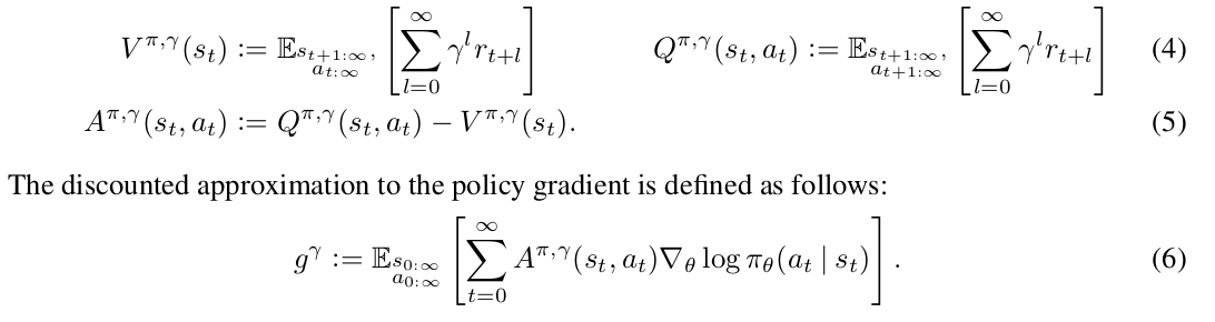
Note that  is a biased estimator of
  but as they claim previous works have studied to “reduce variance by downweighting rewards corresponding to delayed effects, at the cost of introducing bias”.
The paper’s goal is to find a good estimator of  which is called
  .
.
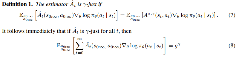
In other word, if is -just, then it helps to construct an unbiased estimator of . Equation (8) just uses the property that the expectation of a sum equals to the sum of expectations.
Now, what other property does have? If we know any property of , it will help us find more easily. The paper proposes one property:

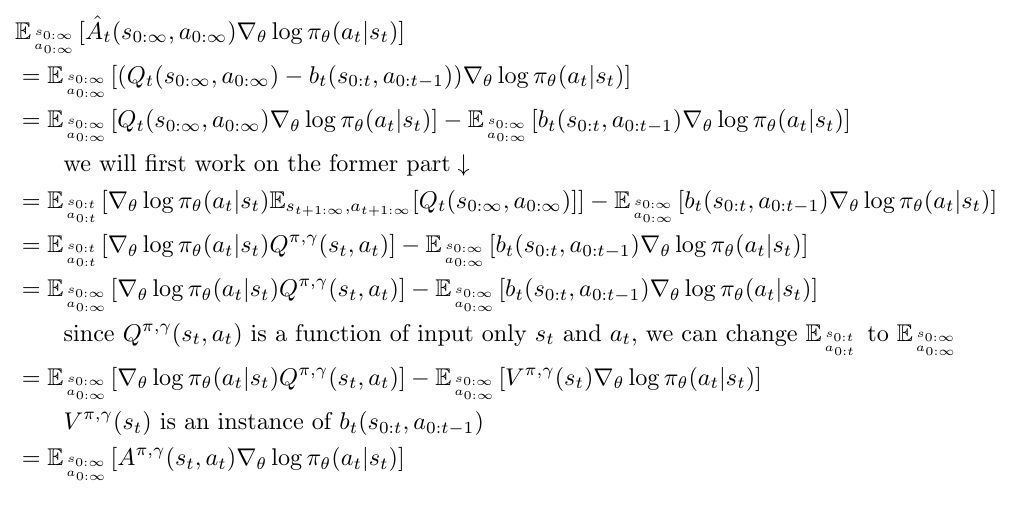
Sketch proof of proposition 1:
First of all, to understand the notations clearly, think that  and
and  are functions with input as the whole trajectory
  . Similarly, think
  as a function with the input as the former part of the trajectory
  .
.
Now, suppose a satisfied such that  where for all
  , then:
Next, they find a good candidate function for , which is  . Only when we know
  is
is  -just. Otherwise
  is a biased estimator of . However, if we can take average of different variations of
  (equation 11, 12, 13, 14, 15, and 16), then we might get a low bias, low variance estimator, which is called
  .
.
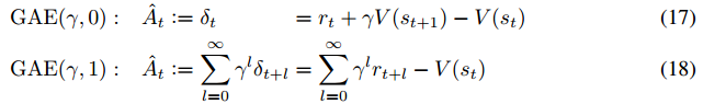
 is -just regardless of the accuracy of (again, this is because
 ![E_{s_{0:\infty}, a_{0:\infty}}[V(s_t) \nabla_\theta \log \pi_\theta (a_t | s_t) ] = 0](https://czxttkl.com/wp-content/ql-cache/quicklatex.com-aa027001db3204456c33147caf9929e0_l3.png "Rendered by QuickLaTeX.com") ). However
). However  is believed (I don’t know how to prove that) to have high variance due to the long sum of rewards. On the other extreme end,
  has low variance but since we are estimating the value function , must be a biased estimator of . with
  would make a trade-off between variance and bias.
Update 2018-11-08
Policy gradient is better illustrated in several recent posts: [11] and [12]
Reference
[1] Reinforcement learning: An introduction
[2] Simple Statistical Gradient-Following Algorithms for Connectionist Reinforcement Learning
[4] Asynchronous Methods for Deep Reinforcement Learning
[5] http://www.breloff.com/DeepRL-OnlineGAE/
[6] HIGH-DIMENSIONAL CONTINUOUS CONTROL USING GENERALIZED ADVANTAGE ESTIMATION
[7] Variance Reduction Techniques for Gradient Estimates in Reinforcement Learning
[9] https://danieltakeshi.github.io/2017/04/02/notes-on-the-generalized-advantage-estimation-paper/
[10] https://www.youtube.com/watch?v=kUiR0RLmGCo
[11] https://lilianweng.github.io/lil-log/2018/04/08/policy-gradient-algorithms.html#soft-actor-critic
[12] https://spinningup.openai.com/en/latest/spinningup/rl_intro3.html#expected-grad-log-prob-lemma
[13] Supplement material of DeepMimic: Example-Guided Deep Reinforcement Learning of Physics-Based Character Skills
[14] Unifying On-Policy and Off-Policy Learning
[15] http://web.stanford.edu/class/cme241/lecture_slides/PolicyGradient.pdf
latex for policy gradient theorem:
![\begin{align*} \nabla \eta(\theta) &= \nabla_\theta v_{\pi} (s_0) \quad \quad \text{performance measure is the value of starting state} \\ &= \nabla_\theta \big[ \sum\limits_{a_0} \pi(a_0|s_0) q(s_0,a_0) \big] \\ &=\sum\limits_{a_0} \big[ \nabla_\theta \pi(a_0|s_0) q(s_0, a_0) + \pi(a_0|s_0) \nabla_\theta q(s_0, a_0) \big] \quad \quad \text{derivative product rule} \\ &= \sum\limits_{a_0} \Big[ \nabla_\theta \pi(a_0|s_0) q(s_0, a_0) + \pi(a_0|s_0) \nabla_\theta \big[ \sum\limits_{s_1,r_0} p(s_1, r_0 |s_0,a_0)(r_0 + \gamma v_\pi(s_1)) \big] \Big] \\ &= \sum\limits_{a_0} \big[ \nabla_\theta \pi (a_0 | s_0) q(s_0, a_0) + \pi(a_0 | s_0) \sum\limits_{s_1} \gamma p(s_1| s_0, a_0) \nabla_\theta v_{\pi}(s_1) \big] \qquad r \text{ has nothing to do with regard to } \theta \\ & \qquad \text{up till now, we have a recursion:} \\ & \qquad \nabla_\theta v_\pi(s_t)= \sum\limits_{a_t} \Big[ \nabla_\theta \pi(a_t|s_t) q(s_t, a_t) + \pi(a_t|s_t) \big[ \sum\limits_{s_{t+1}} \gamma p(s_{t+1}|s_t,a_t) \nabla_\theta v_\pi(s_{t+1}) \big] \Big] \\ &=\sum\limits_{a_0} \Big[ \nabla_\theta \pi (a_0 | s_0) q(s_0, a_0) + \pi(a_0 | s_0) \sum\limits_{s_1} \gamma p(s_1| s_0, a_0) \\ & \qquad \qquad \sum\limits_{a_1} \big[ \nabla_\theta \pi(a_1 | s_1)q(s_1, a_1) + \pi(a_1 | s_1)\sum\limits_{s_2} \gamma p(s_2|s_1, a_1) \nabla_\theta v_{\pi} (s_2) \big] \Big] \\ &=\sum\limits_{a_0} \nabla_\theta \pi (a_0 | s_0) q(s_0, a_0) \\ & \qquad + \gamma \sum\limits_{s_1} \sum\limits_{a_0} p(s_1| s_0, a_0) \pi(a_0 | s_0) \sum\limits_{a_1} \nabla_\theta \pi(a_1 | s_1)q(s_1, a_1) \\ & \qquad + \gamma^2 \sum\limits_{s_2} \sum\limits_{a_1} \sum\limits_{s_1} \sum\limits_{a_0} p(s_2|s_1, a_1) \pi(a_1 | s_1) p(s_1| s_0, a_0) \pi(a_0 | s_0) \nabla_\theta v_{\pi} (s_2) \\ &= \cdots \qquad \text{(keep unrolling using the recursion)}\\ &= \sum\limits_{t=0}^\infty \sum\limits_{s_t} \gamma^t \Pr(s_0 \rightarrow s_t, t, \pi) \sum\limits_{a_t} \nabla_\theta \pi(a_t | s_t) q(s_t, a_t) \qquad \Pr(s_0 \rightarrow s_t, t, \pi) \text{ is the prob. of } s_0 \text{ to } s_t \text{ in } t \text{ steps} \end{align*}](https://czxttkl.com/wp-content/ql-cache/quicklatex.com-8ade309cbfbab77fb5d741c4ea3a7df6_l3.png "Rendered by QuickLaTeX.com")
latex for expectation form rewritten:
![\begin{align*} \nabla \eta(\theta) &= \sum\limits_{t=0}^\infty \sum\limits_{s_t} \gamma^t \Pr(s_0 \rightarrow s_t, t, \pi) \sum\limits_{a_t} \nabla_\theta \pi(a_t | s_t) q(s_t, a_t) \\ &=\sum\limits_{t=0}^\infty \mathbb{E}_{s_t \sim \Pr(s_0 \rightarrow s_t, t, \pi)}[\sum\limits_{a_t} \gamma^t \nabla_\theta \pi(a_t | s_t) q(s_t, a_t) ] \\ &=\sum\limits_{t=0}^\infty \mathbb{E}_{s_t \sim \Pr(s_0 \rightarrow s_t, t, \pi)} [\sum\limits_{a_t} \gamma^t \pi(a_t | s_t) q(s_t, a_t) \frac{\nabla_\theta \pi(a_t | s_t)}{\pi(a_t | s_t)} ] \\ &=\sum\limits_{t=0}^\infty \mathbb{E}_{s_t \sim \Pr(s_0 \rightarrow s_t, t, \pi) \atop a_t \sim \pi(a_t | s_t) \quad}[ \gamma^t q(s_t, a_t) \frac{\nabla_\theta \pi(a_t | s_t)}{\pi(a_t | s_t)}] \\ &=\sum\limits_{t=0}^\infty \mathbb{E}_{s_t \sim \Pr(s_0 \rightarrow s_t, t, \pi) \atop a_t \sim \pi(a_t | s_t) \quad}[ \gamma^t q(s_t, a_t) \nabla_\theta \log \pi(a_t | s_t)] \qquad \nabla \log(x) = \frac{\nabla x}{x} \\ &=\mathbb{E}_{\pi}[ \sum\limits_{t=0}^\infty \gamma^t q(s_t, a_t) \nabla_\theta \log \pi(a_t | s_t)] \\ &=\mathbb{E}_{\pi}[ \sum\limits_{t=0}^\infty \gamma^t G_t \nabla_\theta \log \pi(a_t | s_t)] \end{align*}](https://czxttkl.com/wp-content/ql-cache/quicklatex.com-d532fc2a9f8b3c450bf990553854353e_l3.png "Rendered by QuickLaTeX.com")
latex for adding baseline is still unbiased estimator:
![\begin{align*} &\mathbb{E}_{s_{0:T}, a_{0:T}} [ \sum\limits_{t=0}^T \gamma^t (G_t - b(s_t)) \nabla_\theta \log \pi(a_t | s_t)] \\ =& \mathbb{E}_{s_{0:T}, a_{0:T}} [ \sum\limits_{t=0}^T \gamma^t G_t \nabla_\theta \log \pi(a_t | s_t)] - \mathbb{E}_{s_{0:T}, a_{0:T}}[ \sum\limits_{t=0}^T \gamma^t b(s_t) \nabla_\theta \log \pi (a_t | s_t) ] \\ =& \mathbb{E}_{s_{0:T}, a_{0:T}} [ \sum\limits_{t=0}^T \gamma^t G_t \nabla_\theta \log \pi(a_t | s_t)] - \sum\limits_{t=0}^T \mathbb{E}_{s_{0:T}, a_{0:T}}[ \gamma^t b(s_t) \nabla_\theta \log \pi (a_t | s_t) ] \qquad \text{exp. of sum equals to sum of exp.}\\ =& \mathbb{E}_{s_{0:T}, a_{0:T}} [ \sum\limits_{t=0}^T \gamma^t G_t \nabla_\theta \log \pi(a_t | s_t)] - \sum\limits_{t=0}^T \mathbb{E}_{s_{t}, a_{t}}[ \gamma^t b(s_t) \nabla_\theta \log \pi (a_t | s_t) ] \qquad \text{remove irrelevant variables in each exp.}\\ =& \mathbb{E}_{s_{0:T}, a_{0:T}} [ \sum\limits_{t=0}^T \gamma^t G_t \nabla_\theta \log \pi(a_t | s_t)] - \sum\limits_{t=0}^T \sum\limits_{s_{t}} \sum\limits_{a_{t}} p(s_t, a_t) \gamma^t b(s_t) \nabla_\theta \log \pi (a_t | s_t) \qquad \text{expectation form} \rightarrow \text{discrete sum} \\ =& \mathbb{E}_{s_{0:T}, a_{0:T}} [ \sum\limits_{t=0}^T \gamma^t G_t \nabla_\theta \log \pi(a_t | s_t)] - \sum\limits_{t=0}^T \sum\limits_{s_{t}} \sum\limits_{a_{t}} p(s_t) \pi(a_t|s_t) \gamma^t b(s_t) \frac{\nabla_\theta \pi (a_t | s_t)}{\pi(a_t | s_t) } \qquad \text{rule of probability} \\ =& \mathbb{E}_{s_{0:T}, a_{0:T}} [ \sum\limits_{t=0}^T \gamma^t G_t \nabla_\theta \log \pi(a_t | s_t)] - \sum\limits_{t=0}^T \sum\limits_{s_{t}} \gamma^t b(s_t) p(s_t) \sum\limits_{a_{t}} \nabla_\theta \pi (a_t | s_t) \\ =& \mathbb{E}_{s_{0:T}, a_{0:T}} [ \sum\limits_{t=0}^T \gamma^t G_t \nabla_\theta \log \pi(a_t | s_t)] - \sum\limits_{t=0}^T \sum\limits_{s_{t}} \gamma^t b(s_t) p(s_t) \nabla_\theta \sum\limits_{a_{t}} \pi (a_t | s_t) \\ =& \mathbb{E}_{s_{0:T}, a_{0:T}} [ \sum\limits_{t=0}^T \gamma^t G_t \nabla_\theta \log \pi(a_t | s_t)] - \sum\limits_{t=0}^T \sum\limits_{s_{t}} \gamma^t b(s_t) p(s_t) \nabla_\theta 1 \\ =& \mathbb{E}_{s_{0:T}, a_{0:T}} [ \sum\limits_{t=0}^T \gamma^t G_t \nabla_\theta \log \pi(a_t | s_t)] \\ =& \nabla \eta(\theta) \end{align*}](https://czxttkl.com/wp-content/ql-cache/quicklatex.com-b260de314aa5bf15c7507b755c32d260_l3.png "Rendered by QuickLaTeX.com")
latex for sketch proof of proposition 1:
![\begin{align*} &\mathbb{E}_{s_{0:\infty} \atop a_{0:\infty}} [\hat{A}_t(s_{0:\infty}, a_{0:\infty}) \nabla_\theta \log \pi_\theta(a_t | s_t) ] \\ &= \mathbb{E}_{s_{0:\infty} \atop a_{0:\infty}} [(Q_t(s_{0:\infty}, a_{0:\infty}) - b_t(s_{0:t}, a_{0:t-1})) \nabla_\theta \log \pi_\theta(a_t | s_t)] \\ &= \mathbb{E}_{s_{0:\infty} \atop a_{0:\infty}}[Q_t(s_{0:\infty}, a_{0:\infty}) \nabla_\theta \log \pi_\theta(a_t | s_t)] - \mathbb{E}_{s_{0:\infty} \atop a_{0:\infty}}[b_t(s_{0:t}, a_{0:t-1}) \nabla_\theta \log \pi_\theta(a_t | s_t)] \\ &\qquad \text{we will first work on the former part} \downarrow \\ &= \mathbb{E}_{s_{0:t} \atop a_{0:t}}[\nabla_\theta \log \pi_\theta(a_t | s_t) \mathbb{E}_{s_{t+1:\infty}, a_{t+1:\infty}} [Q_t(s_{0:\infty}, a_{0:\infty})] ] - \mathbb{E}_{s_{0:\infty} \atop a_{0:\infty}}[b_t(s_{0:t}, a_{0:t-1}) \nabla_\theta \log \pi_\theta(a_t | s_t)] \\ &= \mathbb{E}_{s_{0:t} \atop a_{0:t}}[\nabla_\theta \log \pi_\theta(a_t | s_t) Q^{\pi, \gamma}(s_t, a_t)] - \mathbb{E}_{s_{0:\infty} \atop a_{0:\infty}}[b_t(s_{0:t}, a_{0:t-1}) \nabla_\theta \log \pi_\theta(a_t | s_t)] \\ &= \mathbb{E}_{s_{0:\infty} \atop a_{0:\infty}}[\nabla_\theta \log \pi_\theta(a_t | s_t) Q^{\pi, \gamma}(s_t, a_t)] - \mathbb{E}_{s_{0:\infty} \atop a_{0:\infty}}[b_t(s_{0:t}, a_{0:t-1}) \nabla_\theta \log \pi_\theta(a_t | s_t)] \\ &\qquad \text{since } Q^{\pi, \gamma}(s_t, a_t) \text{ is a function of input only } s_t \text{ and } a_t \text{, we can change } \mathbb{E}_{s_{0:t} \atop a_{0:t}} \text{ to } \mathbb{E}_{s_{0:\infty} \atop a_{0:\infty}} \\ &= \mathbb{E}_{s_{0:\infty} \atop a_{0:\infty}}[\nabla_\theta \log \pi_\theta(a_t | s_t) Q^{\pi, \gamma}(s_t, a_t)] - \mathbb{E}_{s_{0:\infty} \atop a_{0:\infty}}[V^{\pi, \gamma}(s_t) \nabla_\theta \log \pi_\theta(a_t | s_t)] \\ &\qquad V^{\pi, \gamma}(s_t) \text{ is an instance of } b_t(s_{0:t}, a_{0:t-1}) \\ &= \mathbb{E}_{s_{0:\infty} \atop a_{0:\infty}} [A^{\pi, \gamma}(s_t, a_t) \nabla_\theta \log \pi_\theta(a_t | s_t) ] \end{align*}](https://czxttkl.com/wp-content/ql-cache/quicklatex.com-fa43561b5bd4e04c093fa2ab3b2d81b9_l3.png "Rendered by QuickLaTeX.com")