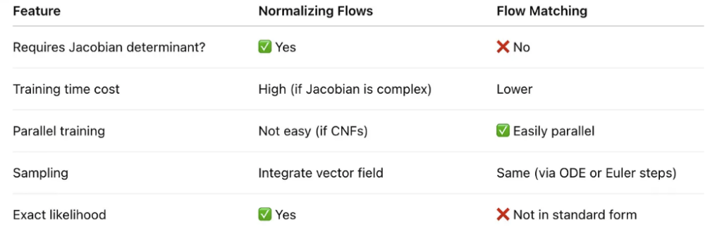
In a previous post, we discussed an earlier generative modeling called Normalizing Flows [1]. However, Normalizing Flows has its own limitations: (1) it requires the flow mapping function  to be invertible. This limits choices of potential neural network architectures to instantiate , because being invertible means that hidden layers must have the exact same dimensionality as the input. (2) computing the log of determinant of the jacobian matrix of is expensive, usually in
  time complexity.
Flow matching is a more recent developed generative modeling technique with lower training cost (see the comparison between Normalizing Flows vs Flow Matching in [2] and a more mathematical introduction of how Flow Matching evolved from Normalizing Flows [6]). In this post, we are going to introduce it. Two materials help me understand flow matching greatly: (1) neurips flow matching tutorial [3] (2) an MIT teaching material [4]
Flow Matching
Motivation
We start from the motivation. Suppose  represents the target space we want to generate (e.g., all dog pictures with
  representing the image dimension). The goal of generative modeling is to learn the real target distribution
  . To enable generating different targets stochastically, the goal usually becomes to learn the transformation from an initial random distribution
  (e.g., Gaussian) the real data distribution .
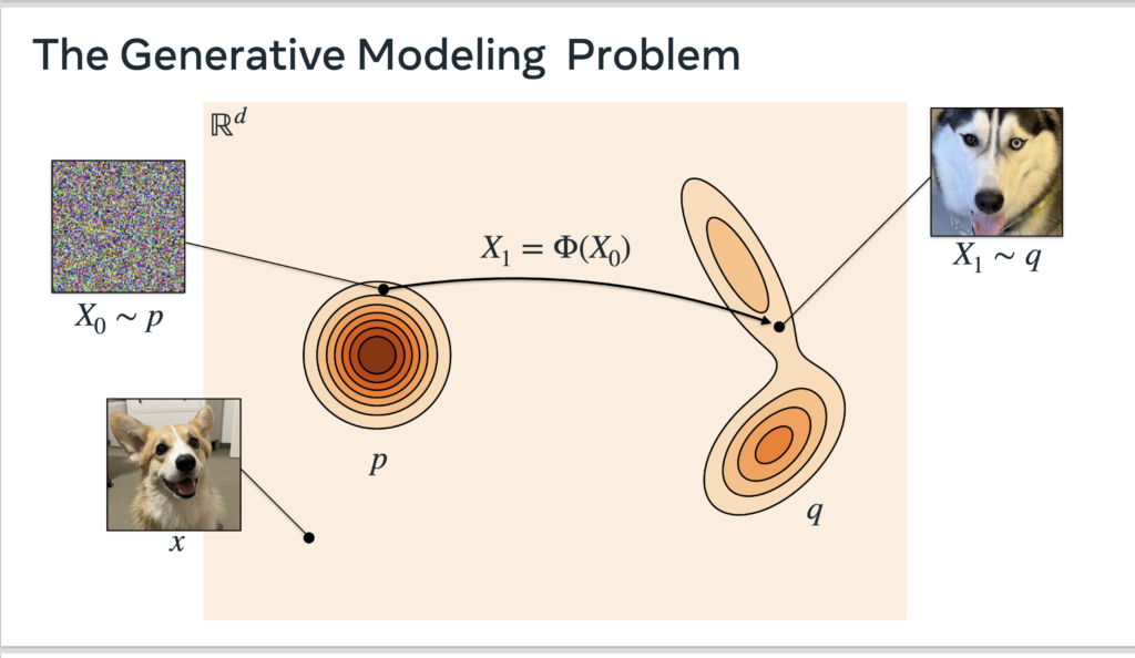
A straightforward method is GAN [5]. However, GAN faces various training instability issues and cannot give the likelihood of a data point, while Flow Matching can address both pain points.
Ordinary Differential Equations (ODE)
ODE describes how a system changes over time. An ODE is defined as:

where ![X: [0, 1] \rightarrow \mathbb{R}^d](https://czxttkl.com/wp-content/ql-cache/quicklatex.com-f9c7da8f7dbe3f55383de3daa935b5c9_l3.png "Rendered by QuickLaTeX.com") . In natural language, we say that
. In natural language, we say that  is a variable representing any point in the -dimensional system at time
  , where each dimension is between 0 and 1. At a given time ( is also between 0 and 1), should move in the direction of
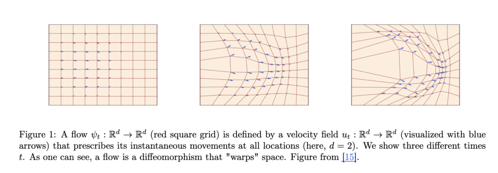
  , which we call the velocity. is also a -dimensional vector. The solution of an ODE is called flow,
  , which tells you where an initial point will be at time . Hence ‘s input is an -dimensional point and output is also an -dimensional point. The ODE above can be rewritten with :

The example below shows how a system moves – the red square grid is the flow, describing each initial point’s “landing” point at time , and the blue arrow is the velocity at time .
 The goal of flow matching is to learn a velocity function
  such that
  and
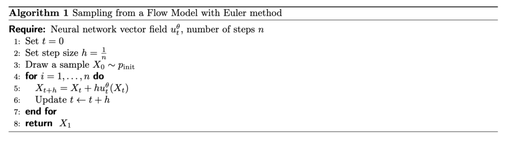
and  . With a known/learned velocity function, you can easily simulate how the system changes, which is equivalent to the flow function :
Conditional / Marginal Probability Path, Conditional and Marginal Velocity Fields
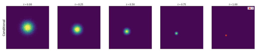
This section is the most mathematical-heavy one. We first introduce the concept of conditional probability path,  . In natural language, means the distribution of the position of a point at time if that point starts from
  at time 0 and ends at exactly
  (i.e., a delta distribution at ) at time 1, where is any data sampled from the target distribution
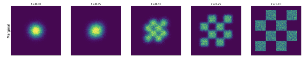
  . Therefore, the marginal probability path
  can be described as:
 .
.
simply describes the position distribution of the whole system at time , given the initial distribution is and the end distribution is .
The diagram below describes an example of conditional probability path : it starts from a 2D gaussian distribution and ends at a particular position marked by the red dot.
The diagram below describes an example of marginal probability path : it starts from a 2D gaussian distribution and ends at a chessboard-patterned distribution.
Deriving from the concepts of conditional/marginal probability path, we can also have conditional and marginal velocity field, defined as:
Conditional velocity field: 
Marginal velocity field: 
The formula of marginal velocity field needs a bit work to be proved. We use the rest of this section to prove that.
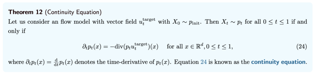
First, we introduce a theorem called Continuity Equation:
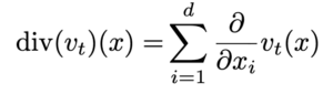
 where the divergence operator is defined as:
In natural language, this equation says that the change of marginal probability path w.r.t. time is equal to the negative divergence of  . The same theorem can also be applied to the conditional probability path:
  .
.
Now we can show that:

By the last two equations, we proved the relationship between the marginal and conditional velocity fields:
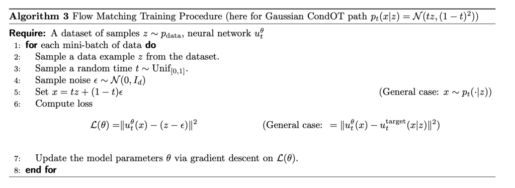
Training a Practical Flow Matching model
To reiterate the motivation of flow matching: our goal is to learn a velocity function such that and . Therefore, the ultimate goal should be:
![\mathcal{L}_{FM}(\theta) = \mathbb{E}_{t\sim Unif[0,1], x\sim p_t} \left[ \left\Vert \mu_t^\theta(x)-\mu_t(x) \right\Vert^2 \right] = \mathbb{E}_{t\sim Unif[0,1], z\sim p_{data}, x\sim p_t(\cdot|z)} \left[ \left\Vert \mu_t^\theta(x)-\mu_t(x) \right\Vert^2 \right]](https://czxttkl.com/wp-content/ql-cache/quicklatex.com-8d442e13a50791c6da29960192c9f0db_l3.png "Rendered by QuickLaTeX.com")
Recall in the section above that , which involves an integration operator and thus is intractable. Interestingly, we can prove that ![\mathcal{L}_{FM}(\theta)=\mathbb{E}_{t\sim Unif[0,1], z\sim p_{data}, x\sim p_t(\cdot|z)} \left[ \left\Vert \mu_t^\theta(x)-\mu_t(x) \right\Vert^2 \right] = \mathbb{E}_{t\sim Unif[0,1], z\sim p_{data}, x\sim p_t(\cdot|z)} \left[ \left\Vert \mu_t^\theta(x)-\mu_t(x|z) \right\Vert^2 \right] = \mathcal{L}_{CFM}(\theta)](https://czxttkl.com/wp-content/ql-cache/quicklatex.com-1e72627ef5ceb9eb41cd75389f19eec3_l3.png "Rendered by QuickLaTeX.com") . Therefore, we can explicitly regress our parameterized velocity function against a tractable conditional vector field. This proof can be found in Theorem 18 in [4].
. Therefore, we can explicitly regress our parameterized velocity function against a tractable conditional vector field. This proof can be found in Theorem 18 in [4].
The exact form of  depends on what family of probability path we choose. One particularly popular probability path is the Gaussian probability path. We can define
  and
and  to be two continuously differentiable, monotonic functions with
  and
and  . We can verify that the conditional Gaussian probability path parameterized by and ,
  , satisfies the definition of a conditional probability path: at time 0,
  and
and  . Note that, with the Gaussian conditional probability path, we can simulate the position of
  :
:  , where
  . We can then prove that
  (see detailed proof in Example 11 in [4]).
With all these intermediate artifacts, we can derive the loss function:
![\begin{align*} \mathcal{L}_{CFM}(\theta) &= \mathbb{E}_{t\sim Unif[0,1], z\sim p_{data}, x\sim p_t(\cdot|z)} \left[ \left\Vert \mu_t^\theta(x)-\mu_t(x|z) \right\Vert^2 \right] \\ &= \mathbb{E}_{t\sim Unif[0,1], z\sim p_{data}, x\sim p_t(\cdot|z)} \left[ \left\Vert \mu_t^\theta(x)-\left(\dot{\alpha_t}-\frac{\dot{\beta_t}}{\beta_t}\alpha_t \right)z - \frac{\dot{\beta_t}}{\beta_t}x \right\Vert^2 \right] \\ &(\text{let } x=\alpha_t z + \beta_t \epsilon) \\ &= \mathbb{E}_{t\sim Unif[0,1], z\sim p_{data}, x\sim p_t(\cdot|z)} \left[ \left\Vert \mu_t^\theta(\alpha_t z + \beta_t \epsilon) - (\dot{\alpha_t} z + \dot{\beta_t} \epsilon) \right\Vert^2 \right] &(\text{special case: } alpha_t=t, \beta_t=1-t) \\ &=\mathbb{E}_{t\sim Unif[0,1], z\sim p_{data}, x\sim p_t(\cdot|z)} \left[ \left\Vert \mu_t^\theta(tz+(1-t)\epsilon) - (z- \epsilon) \right\Vert^2 \right] \end{align*}](https://czxttkl.com/wp-content/ql-cache/quicklatex.com-6d2afce51e8290a674829c7bfe31e112_l3.png "Rendered by QuickLaTeX.com")
References
[1] https://czxttkl.com/2021/11/15/normalizing-flows/
[2] https://medium.com/@noraveshfarshad/flow-matching-and-normalizing-flows-49c0b06b2966
[3] https://neurips.cc/virtual/2024/tutorial/99531
[4] https://diffusion.csail.mit.edu/docs/lecture-notes.pdf
[5] https://czxttkl.com/2020/12/24/gan-generative-adversarial-network/
[6] https://mlg.eng.cam.ac.uk/blog/2024/01/20/flow-matching.html


 and
and  ,
,  ,
,  , which transform token embeddings
  into a projected latent space.
 is the attention matrix.
  represents how much attention token
  should pay for
  . In normal LLM tasks, we will apply a causal mask so that only
  is valid, because a token can only pay attention to all previous tokens. The softmax() operator is applied per-row of
  .
. represents the weighted values from other tokens per position.
  to
to  ). We omit the part after self-attention.
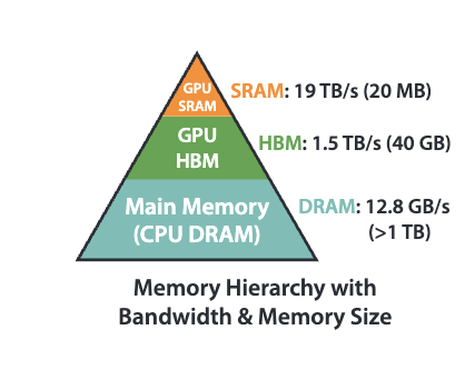 In standard self-attention, it requires
  HBM accesses, because we need to load
  ,
,  , and
, and  from HBM and we need to read/write of
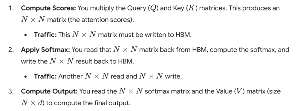
  . A detailed breakdown of standard self-attention HBM accesses is as below (illustrated by Gemini):
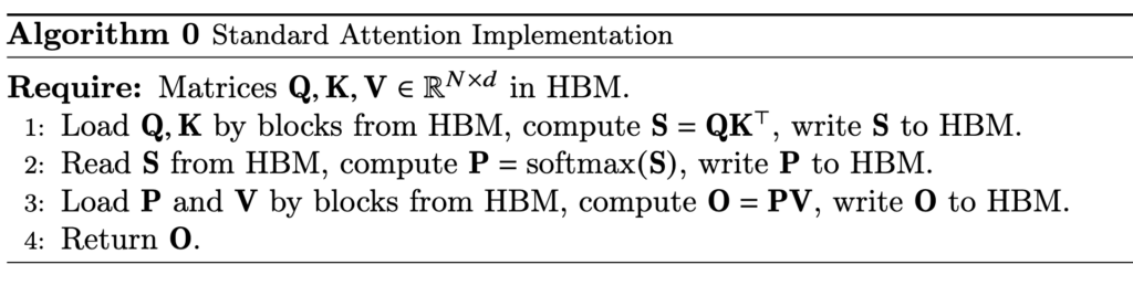
 Let’s dive into the step of computing softmax. Even computing softmax has many details. First, in real world, we usually need to compute a safe softmax version, where we subtract each input to the softmax with the maximum input to avoid potential overflow. (Diagrams from [3])
 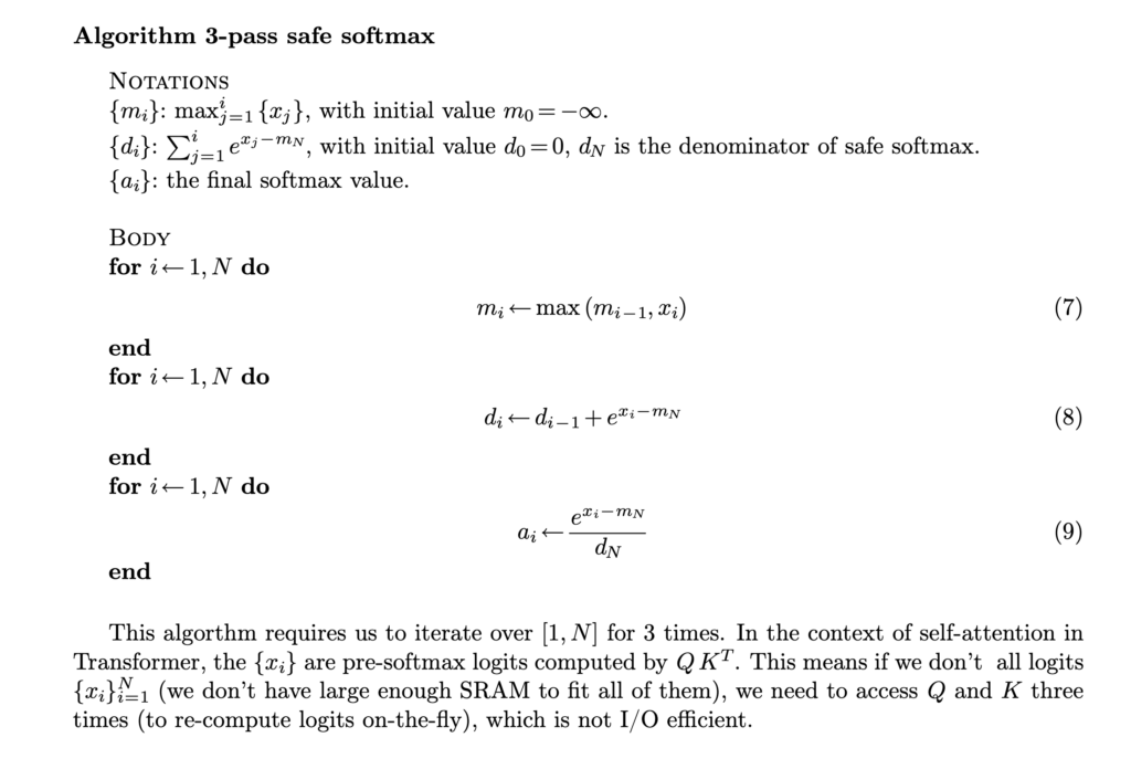 In its vanilla implementation, we need to have three passes: the first pass computes the maximum of the input, the second pass computes the denominator of the softmax, and the third pass computes the actual softmax. Asymptotically these three steps require
  time but in reality the constant factor of the
  computation is also important. SRAM is typically too small to hold the
  result. So we either need to save
  , depending whichever is faster. That means this three-passes safe softmax algorithm does require
  computation time / accesses to HBM. It turns out that we can turn the 3-passes algorithm into 2-passes. This is something called online softmax. As we traverse each
  , we can record the maximum value so far and the accumulative softmax denominator. The accumulative softmax denominator from the previous
  can be easily scaled whenever a new maximum is found at
 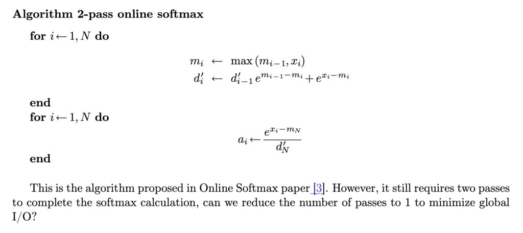 With this 2-pass online softmax algorithm, self-attention can also be computed in two-passes:
 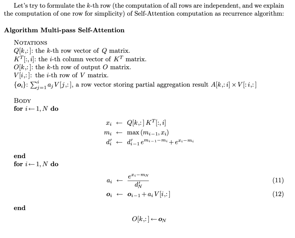 However, we can do better by finding that
  can also be computed “online” together with the running maximum value
  and running accumulative softmax denominator
  .
. 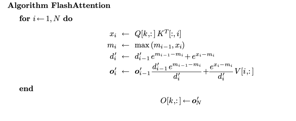 That’s how we end up with FlashAttention which requires one pass to compute the output vectors!
 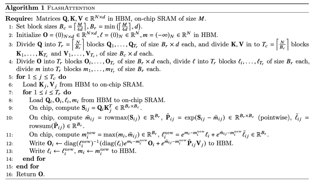 In reality, a further optimization is to load Q/K/V in blocks so that the blocks of Q, K, V, and O can occupy roughly the full SRAM memory at one time. That’s why we see block size is set at
  or
or  in the algorithm.
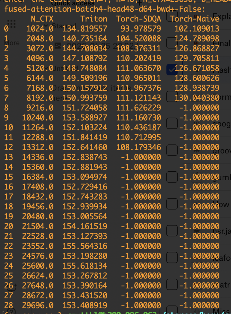
 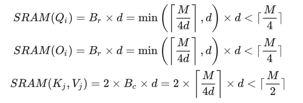 Now, we examine how to do backward computation in FlashAttention. We start from examining the standard attention backward pass:
 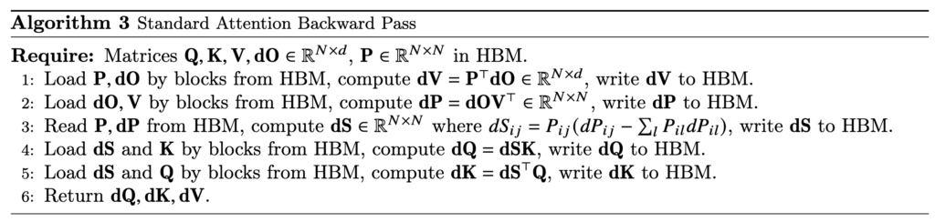 (To clarify the notations,
  is the gradient of the loss
  with respect to the attention output matrix, i.e.,
  , which has the same shape as
  ,
,  , and
, and  . We also assume
  , due to matrix calculus rules, we have
  .
. because it will be used in computing
  .
. . There is a well-known mathematical result stating that the Jacobian matrix of softmax can be computed by
 ![J(P_i) = J\left(softmax(S_i)\right)=\left[ \frac{\partial P_i}{\partial s_{i1}}, \cdots, \frac{\partial P_i}{\partial s_{iN}} \right]=diag(P_i) - P_i P_i^T](https://czxttkl.com/wp-content/ql-cache/quicklatex.com-7d889816bffd9d21c3231865b9724587_l3.png "Rendered by QuickLaTeX.com") , where
, where  is a row of
  . [Note: while
  is a row of
  is actually a scalar, an inner product, while
  is a matrix, an outer product, of the two vectors.]
 and
and  .
. ,
,  can be computed and prestored in HBM via
  and
and  :
: 
 because one full inner loop (starting from line 7 in Algorithm 1) needs to load the full
  ), and the outer loop (line 5 in Algorithm 1) needs to perform
  times (
 ). Another good reference of IO complexity analysis can be found in [4]
 can be greatly smaller than
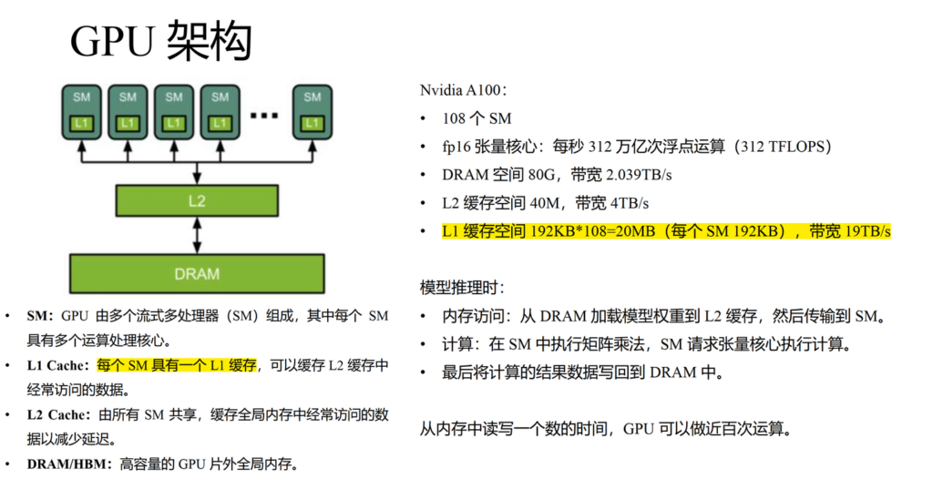
  . First of all, we need to clarify that
  should represent the L1 cache size of one streaming multiprocessor (SM) in a GPU. Taking A100 as an example, one SM has 192KB L1 cache. So FlashAttention will probably have advantage of IO complexity when
  64, 128, or 256 but has no advantage when
  .
.  Let’s also summarize the total memory footprint required by standard attention vs FlashAttention: 1. standard attention: it needs to store
  space. Overall, the memory footprint of FlashAttention is only
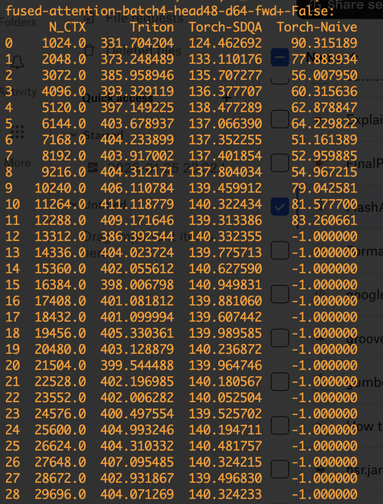


 , a length
  being the i-th element. Each word has its corresponding embedding
  , where
  , a
, a  , the word (
 )’s output is a weighted sum of all values of other words in the sequence, where the weights are determined by the self-attention mechanism:


 ,
,  and
and  are the dimension indices of the positional encoding hence
  .
. makes
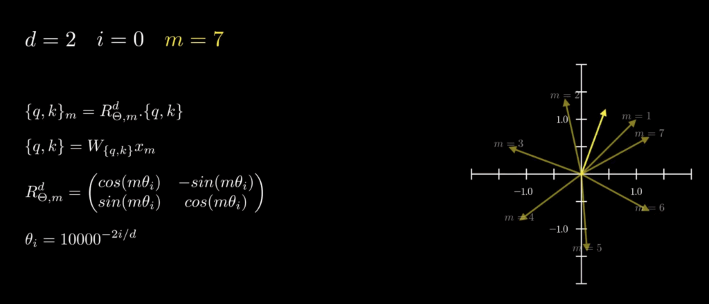
makes  a bit chaotic. In the motivational example from [4], suppose
  , then at different positions 0 ~ 7,
  , making LLMs hard to generalize.


 by default
 ,
, 
 , their (unnormalized) attention scores depend on the position difference
  . As
. As ![\mathbf{q}_t^T \mathbf{k}_s = \left(\mathbf{R}^{d}_{\Theta, t} \mathbf{W}_q \mathbf{x}_t \right)^T \left(\mathbf{R}^{d}_{\Theta, s} \mathbf{W}_k \mathbf{x}_s \right) \newline\qquad =\mathbf{x}^T_t \mathbf{W}_q \mathbf{R}^{d}_{\Theta, t-s} \mathbf{W}_k \mathbf{x}_s \newline\qquad = Re\left[\sum\limits_{i=0}^{d/2-1} \mathbf{q}_{[2i:2i+1]} \mathbf{k}^*_{[2i:2i+1]} e^{i(t-s)\theta_{i}} \right]\newline \qquad \text{decrease as t-s increases}](https://czxttkl.com/wp-content/ql-cache/quicklatex.com-d94c4f09c13f52eb6323ff2ef3d152a1_l3.png "Rendered by QuickLaTeX.com")
 , post-train a context window
  , and need to inference with a longer context window
  . We assume
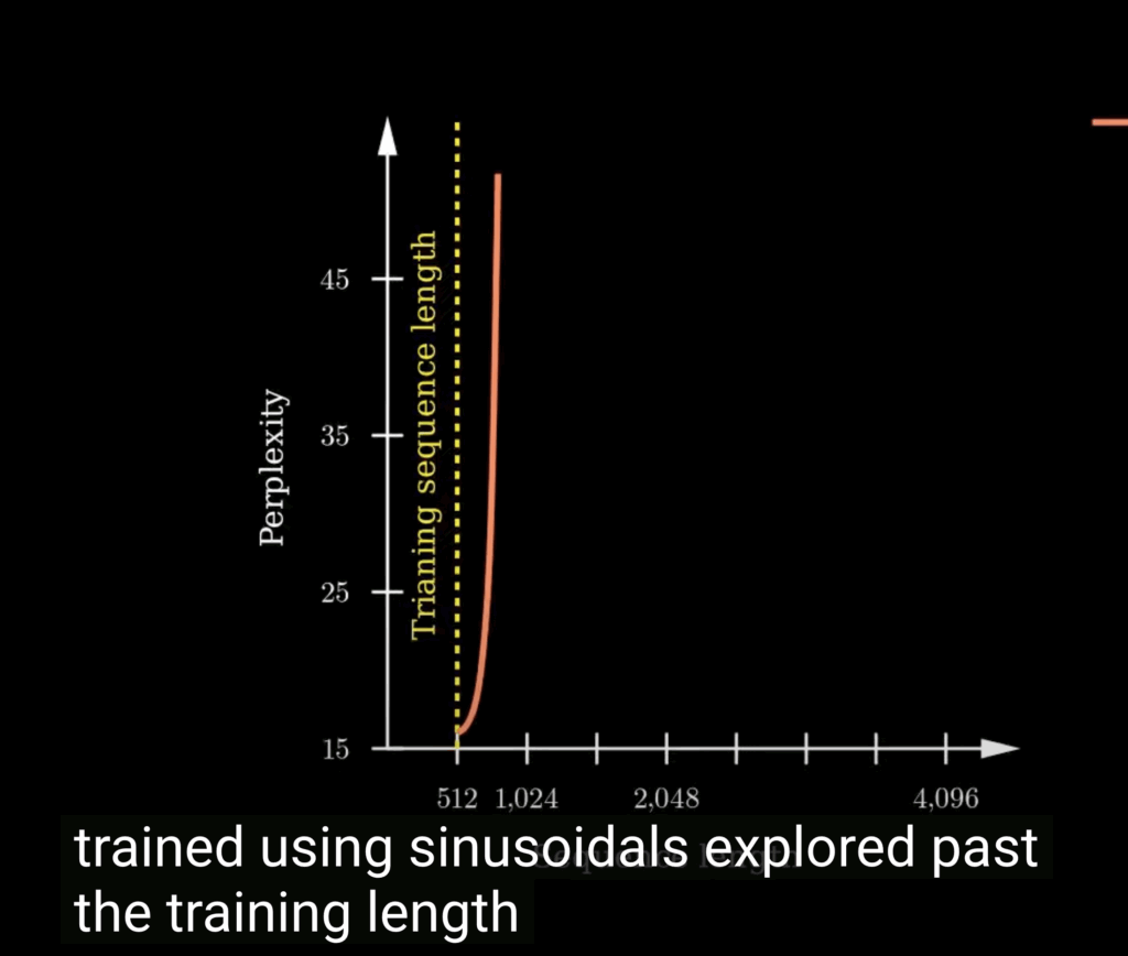
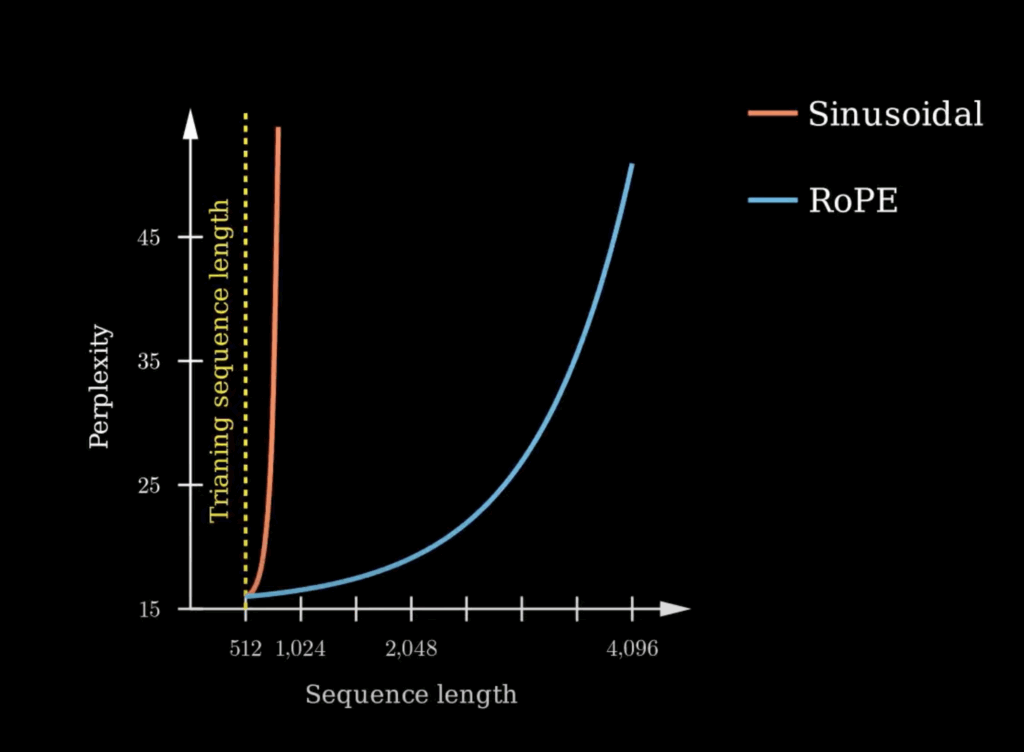
  . Without any remedies, perplexity will shoot up outside
  and
and  , post-training RoPE with
  and
and  has the best extrapolation performance, followed by
  , then followed by
  and
and 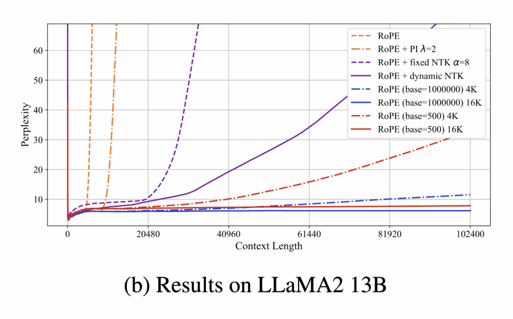
 can improve extrapolation. As we introduced, when computing attention scores, RoPE is essentially rotating embeddings by different angles – for any two positions
  , where
  ,
,  . The larger the base
  ,
,  so that the model has learned representation for every possible relative position difference
  ), the best compromise we can make in post-training is to let as many embedding dimensions as possible to have small periods (
 ). As such, the model will see full cycles of rotations of those dimensions within
  . This means that when
  ,
,  . Therefore, there will be 92 dimensions whose periods can fit into the 4k context length while the remaining 36 dimensions’ periods are longer than 4k. If we change
  increases). Therefore, in test time, even we see a relative position difference
  that could happen in large
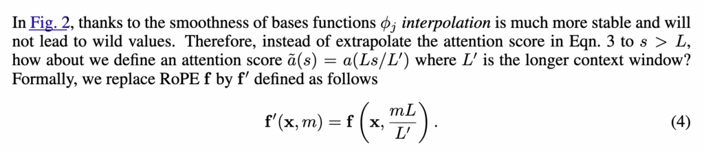
 ) contains compressed information from all previous segments and is updated after each segment to carry new information over. Therefore, in theory, the model can extend to infinite context.
 measures the amount of information obtained about one random variable by observing the other random variable:

 and hypothesize data is generated by a latent process
  , starting from a latent code
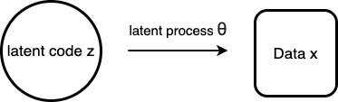
 , sometimes called the “log evidence”. Let
  to describe the posterior probability of
  to describe the joint probability of
  to approximate
  being learnable parameters.
  can be rewritten into [see 6, page 22-23 for derivation]:
 .
. , the evidence lower bound (ELBO). We have
  because
  . Therefore, we can maximize ELBO w.r.t.
 ![log p_\theta(x) \geq - KL\left(q_\phi(z|x) \Vert p_\theta(x, z)\right) = \newline \mathbb{E}_{z\sim q_\phi(z|x)}\left[ log p_\theta(x|z)\right] - KL\left( q_\phi(z|x) \Vert p(z) \right)](https://czxttkl.com/wp-content/ql-cache/quicklatex.com-c4e9ded405df8f5d13f8a29d89cb7445_l3.png "Rendered by QuickLaTeX.com") ,
, is the prior for the latent code (e.g., standard normal distributions). In VAE, we also use a deterministic neural network to approximate
  . Overall,
 ![\mathbb{E}_{z\sim q_\phi(z|x)}\left[ log q_{\phi'}(x|z)\right] - KL\left( q_\phi(z|x) \Vert p(z) \right)](https://czxttkl.com/wp-content/ql-cache/quicklatex.com-6b189b2d079ea15bd219f14afeb9ab9a_l3.png "Rendered by QuickLaTeX.com") can be learned by minibatch samples and when ELBO is maximized,
can be learned by minibatch samples and when ELBO is maximized,  (label) in a supervised learning setting. The objective is to encode
![I(z;y) - \beta I(z;x) \geq \mathbb{E}_{z\sim q_{\phi}(z|x)}\left[ log q_{\phi'}(y|z) \right]-\beta KL\left(q_\phi(z|x) \Vert p(z)\right),](https://czxttkl.com/wp-content/ql-cache/quicklatex.com-7f01b74d310debf5d8608bfdb75f0a63_l3.png "Rendered by QuickLaTeX.com")
 is the decoder network.
 , which is known at training time but unknown at testing time. The authors of [1] propose to learn two policies:
  for exploring environments with the goal to collect as much information about the environment as possible, and
  for exploiting an environment with a known encoded tensor
  , an encoder to encode environment tensor
  (available in training time) or
  , a variational encoder which converts the trajectory generated by
  will be learned to match
  in training time. Once
  , and
, and  are learned, at testing time, we can run
  , use
, use ![\text{minimize} \qquad I(z;u) \newline \text{subject to} \quad \mathbb{E}_{z \sim F_{\psi}(z|\mu)}\left[ V^{\pi_\theta^{task}}(z;\mu)\right]=V^*(\mu) \text{ for all } \mu](https://czxttkl.com/wp-content/ql-cache/quicklatex.com-d4f0b6a04603baee6f6cffcd0c405b09_l3.png "Rendered by QuickLaTeX.com")
 set as a hyperparameter [8]:
 ![\text{maximize}_{\psi, \theta}\quad \mathbb{E}_{\mu \sim p(\mu), z\sim F_{\psi}(z|\mu)}\left[V^{\pi_\theta^{task}}(z;\mu) \right] - \lambda I(z;\mu)](https://czxttkl.com/wp-content/ql-cache/quicklatex.com-14c643f47ee86cda0de04cd5656648fe_l3.png "Rendered by QuickLaTeX.com")
 is
is  , which has an analytic form when the prior
  :
:![I(\tau^{exp};z) = H(z) - H(z|\tau^{exp}) \geq H(z) + \mathbb{E}_{\mu, z\sim F_\psi, \tau^{exp}\sim \pi^{exp}}\left[ q_\omega(z|\tau^{exp}) \right]](https://czxttkl.com/wp-content/ql-cache/quicklatex.com-469e9c83627a52bb29fc69a25b776eb9_l3.png "Rendered by QuickLaTeX.com")
 , is greater than or equal to 0. )
 is learned to match
 ![\mathbb{E}_{\mu, z\sim F_\psi, \tau^{exp}\sim \pi^{exp}}\left[ q_\omega(z|\tau^{exp}) \right]](https://czxttkl.com/wp-content/ql-cache/quicklatex.com-c5fa0e78a60ee5ee658bc9460e1d7145_l3.png "Rendered by QuickLaTeX.com") , we can optimize
, we can optimize  , which is exactly the next token prediction distribution.


 , is:
, is:![\max_{\pi_\theta} \mathbb{E}_{x \sim \mathcal{D}, y\sim \pi_\theta(y|x)}[r_\phi(x,y)] - \beta \mathbb{D}_{KL}[\pi_\theta(y|x) || \pi_{ref}(y|x)],](https://czxttkl.com/wp-content/ql-cache/quicklatex.com-240b38196767f08289ae9f30402a4127_l3.png "Rendered by QuickLaTeX.com")
 but also, in balance, to minimize the KL-divergence from a reference policy
  .
. ![\mathbb{D}_{KL}[\pi_\theta(y|x) || \pi_{ref}(y|x)]=\sum_y \pi_\theta(y|x) \log\frac{\pi_\theta(y|x)}{\pi_{ref}(y|x)} =\mathbb{E}_{y\sim \pi_\theta(y|x)}[\log\frac{\pi_\theta(y|x)}{\pi_{ref}(y|x)}]](https://czxttkl.com/wp-content/ql-cache/quicklatex.com-5ebf661034347ef1a26ee6ad1aea9464_l3.png "Rendered by QuickLaTeX.com") , we have
, we have![\max_{\pi_\theta} \mathbb{E}_{x \sim \mathcal{D}, y\sim \pi_\theta(y|x)}\left[r_\phi(x,y) - \beta (\log \pi_\theta(y|x) - \log \pi_{ref}(y|x)) \right] \newline = \mathbb{E}_{x \sim \mathcal{D}, y\sim \pi_\theta(y|x)}\left[r_\phi(x,y) + \beta \log \pi_{ref}(y|x) - \beta \log \pi_\theta(y|x) \right] \newline \text{because }-\log \pi_\theta(y|x) \text{ is an unbiased estimator of entropy } \mathcal{H}(\pi_\theta)=-\sum_y \pi_\theta(y|x) \log \pi_\theta(y|x), \newline \text{we can transform to equation 2 in [3]} \newline= \mathbb{E}_{x \sim \mathcal{D}, y\sim \pi_\theta(y|x)}\left[r_\phi(x,y) + \beta \log \pi_{ref}(y|x) + \beta \mathcal{H}(\pi_\theta)\right]](https://czxttkl.com/wp-content/ql-cache/quicklatex.com-a33dea15a8c89bf3260776df1cf4d7be_l3.png "Rendered by QuickLaTeX.com")
![\max_{\pi_\theta} \mathbb{E}_{x \sim \mathcal{D}, y\sim \pi_\theta(y|x)}\left[r_\phi(x,y) - \beta (\log \pi_\theta(y|x) - \log \pi_{ref}(y|x)) \right] \newline = \min_{\pi_\theta} \mathbb{E}_{x \sim \mathcal{D}, y\sim \pi_\theta(y|x)} \left[ \log \frac{\pi_\theta(y|x)}{\pi_{ref}(y|x)} - \frac{1}{\beta}r_\phi(x,y) \right] \newline =\min_{\pi_\theta} \mathbb{E}_{x \sim \mathcal{D}, y\sim \pi_\theta(y|x)} \left[ \log \frac{\pi_\theta(y|x)}{\pi_{ref}(y|x)} - \log exp\left(\frac{1}{\beta}r_\phi(x,y)\right) \right] \newline = \min_{\pi_\theta} \mathbb{E}_{x \sim \mathcal{D}, y\sim \pi_\theta(y|x)} \left[ \log \frac{\pi_\theta(y|x)}{\pi_{ref}(y|x)exp\left(\frac{1}{\beta}r_\phi(x,y)\right)} \right] \newline \pi_{ref}(y|x)exp\left(\frac{1}{\beta}r_\phi(x,y)\right) \text{ may not be a valid distribution. But we can define a valid distribution:} \pi^*(y|x)=\frac{1}{Z(x)}\pi_{ref}(y|x)exp\left(\frac{1}{\beta}r_\phi(x,y)\right), \text{ where } Z(x) \text{ is a partition function not depending on } y \newline = \min_{\pi_\theta} \mathbb{E}_{x \sim \mathcal{D}, y\sim \pi_\theta(y|x)} \left[ \log \frac{\pi_\theta(y|x)}{\pi^*(y|x)} \right]](https://czxttkl.com/wp-content/ql-cache/quicklatex.com-abe10cca2808da4aaf2d3f96b11abd12_l3.png "Rendered by QuickLaTeX.com")
 everywhere.
![\max_{\pi_\theta} \mathbb{E}_{x \sim \mathcal{D}, y\sim \pi_\theta(y|x)}\left[\underbrace{r_\phi(x,y) + \beta \log \pi_{ref}(y|x)}_{\text{actual reward function}} + \beta \mathcal{H}(\pi_\theta)\right] \newline s.t. \quad \sum\limits_y \pi_\theta(y|x)=1,](https://czxttkl.com/wp-content/ql-cache/quicklatex.com-806a96f47b9f83798b88f60131252bf1_l3.png "Rendered by QuickLaTeX.com")
 . Note, we are solving a one-step MaxEnt RL problem. So we can use the Lagrangian multipliers method to reach the same solution. See 1hr:09min in [5] for more details.
 . With some arrangement, we can see that this formula entails that the reward function can be represented as a function of
  and
and 
 and a Bradley-Terry model, we know that
 into the logit [7]:
![-\mathbb{E}_{(x, y_w, y_l) \sim \mathcal{D}}\left[\log \sigma \left(r(x, y_w) - r(x, y_l)\right) \right] \newline = -\mathbb{E}_{(x, y_w, y_l) \sim \mathcal{D}}\left[ \log \sigma \left( \left(\beta \log \pi^*_\theta(y_w|x) - \beta \log \pi_{ref} (y_w | x) \right) - \left( \beta \log \pi^*_\theta(y_l |x) - \beta \log \pi_{ref} (y_l | x) \right)\right)\right] \newline = -\mathbb{E}_{(x, y_w, y_l) \sim \mathcal{D}}\left[ \log \sigma \left( \beta \log \frac{\pi^*_\theta(y_w|x)}{\pi_{ref} (y_w | x)} - \beta \log \frac{\pi^*_\theta(y_l |x)}{\pi_{ref} (y_l | x)} \right) \right]](https://czxttkl.com/wp-content/ql-cache/quicklatex.com-f305d09d3d4969371cc4d16552d0e9fe_l3.png "Rendered by QuickLaTeX.com")

![-\mathbb{E}_{(x, y_w, y_l) \sim \mathcal{D}}\left[ \log \sigma \left( \beta \log \frac{\pi^*_\theta(y_w|x)}{\pi_{ref} (y_w | x)} - \beta \log \frac{\pi^*_\theta(y_l |x)}{\pi_{ref} (y_l | x)} \right) \right]](https://czxttkl.com/wp-content/ql-cache/quicklatex.com-ff2bc73960aca346b8a20c8baa04e2f3_l3.png "Rendered by QuickLaTeX.com") , still align the underlying policy to the Bradley-Terry preference probability defined in the token-level MDP? The answer is yes as proved in [3]. We first need to make an interesting connection between the decoding process and multi-step Maximum Entropy RL. (Note, earlier in this post, we have made a connection between on-step Maximum Entropy RL and DPO in the setting of bandits.)
, still align the underlying policy to the Bradley-Terry preference probability defined in the token-level MDP? The answer is yes as proved in [3]. We first need to make an interesting connection between the decoding process and multi-step Maximum Entropy RL. (Note, earlier in this post, we have made a connection between on-step Maximum Entropy RL and DPO in the setting of bandits.) ![\pi^*_{MaxEnt} = \arg\max_\pi \sum_t \mathbb{E}_{(s_t, a_t) \sim \pho_\pi} \left[ r(s_t, a_t) + \beta \mathcal{H}\left(\pi(\cdot | s_t)\right)\right]](https://czxttkl.com/wp-content/ql-cache/quicklatex.com-4d58c569f6261979c4601a0f193caf00_l3.png "Rendered by QuickLaTeX.com") . People have proved the optimal policy can be derived as
. People have proved the optimal policy can be derived as  where
where  and
and  are the corresponding Q-function and V-function in the MaxEnt RL [8]. For any LLM, its decoding policy
  is a softmax over the whole vocabulary. Therefore,
  in terms of an LLM’s decoding process. We could re-arrange the formula to represent per-token reward as:

![-\mathbb{E}_{(x, y_w, y_l) \sim \mathcal{D}} \left[ \log \sigma \left(\beta \sum\limits_{i=1}^{N}\log \frac{\pi_\theta(y_w^i | x, y_{w, <i})}{\pi_{ref}(y_w^i | x, y_{w,<i})} - \beta \sum\limits_{i=1}^M \log \frac{\pi_\theta(y_l^i | x, y_{l, <i})}{\pi_{ref}(y_l^i | x, y_{l,<i})} \right) \right] \newline = -\mathbb{E}_{(x, y_w, y_l) \sim \mathcal{D}}\left[ \log \sigma \left( \beta \log \frac{\pi^*_\theta(y_w|x)}{\pi_{ref} (y_w | x)} - \beta \log \frac{\pi^*_\theta(y_l |x)}{\pi_{ref} (y_l | x)} \right) \right]](https://czxttkl.com/wp-content/ql-cache/quicklatex.com-982b48b23d236150e21ff1c8f0e9f051_l3.png "Rendered by QuickLaTeX.com")


 ; if X and Y are d-separated, then X and Y are independent given Z, denoted as
  . If two nodes are not d-connected, then they are d-separated. There are several rules for determining whether two nodes are d-connected or d-separated [3]. An interesting (and often non-intuitive) example is that in a v-structure like (X3, X4, X5) above: X3 is d-connected (i.e., dependent) to X4 given X5 (i.e., the collider), even though X3 and X4 has no direct edge in between [4].
 . When
  , the conditional independence test will return us
  . Therefore, the identified conditional independence relationship from the data is not entailed by the FCM.
![X_i = \sum\limits_k \alpha_k P_a^k(X_i)+E_i, \;\; i \in [1, N]](https://czxttkl.com/wp-content/ql-cache/quicklatex.com-175e512cfb74f88cb005d0dd0d358d15_l3.png "Rendered by QuickLaTeX.com")

 is not a linear model with Gaussian input and Gaussian noise