Stochastic Variational Inference

Introduction

In this post, we introduce one machine learning technique called stochastic variational inference that is widely used to estimate posterior distribution of Bayesian models. Suppose in a Bayesian model, the model parameters is denoted as a vector $z$ and the observation is denoted as $x$ . According to Bayesian theorem, the posterior distribution of $z$ can be computed as:

$p(z|x)=\frac{p(z,x)}{p(x)}$

$p(x)$ is the probability of observation marginal over all possible model parameters:

$p(x)=\int p(z,x)dz$

$p(x)$ isn’t easy to compute, most of time intractable, because of its integral form. If we are not able to compute $p(x)$ , then we are not able to compute $p(z|x)$ , which is what we want to know. Therefore, we need to come up with a way to approximate $p(z|x)$ . We denote the approximated posterior as $q(z)$ . $q(z)$ is also called the variational distribution hence the name of variational inference.

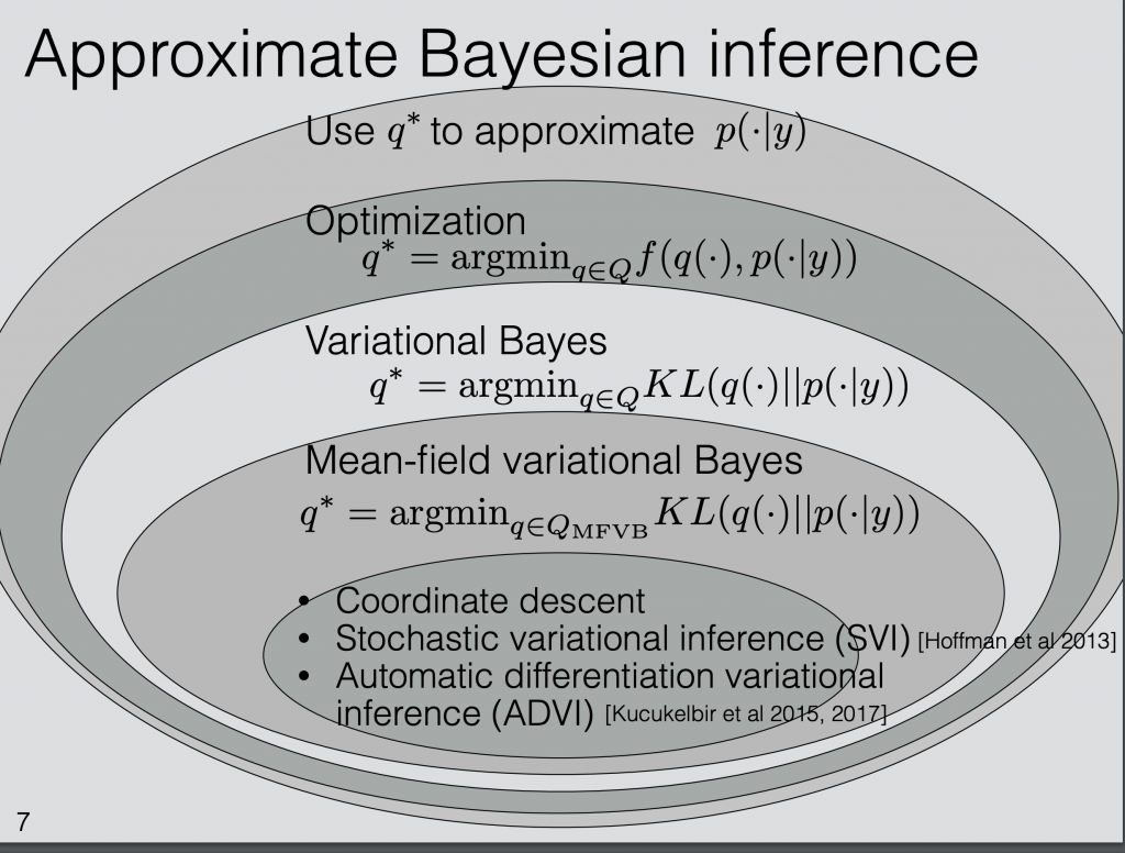
Stochastic variational inference (SVI) is such one method to approximate $p(z|x)$ . From the ICML 2018 tutorial [2], we can see the niche where SVI lies: among all possible ways to approximate $p(z|x)$ , there is a group of algorithms using optimization to minimize the difference between $q^*(\cdot)$ and $p(\cdot|x)$ . Those representing the difference between the two distributions as Kullback-Leibler divergence is called variational inference. If we further categorize based on the family of $q^*$ , there is one particular family called mean-field variational family which is easy to apply variational inference. After all levels of categorization, we arrive at some form of objective function which we sort to minimize. SVI is one optimization method to optimize a defined objective function that pushes $q^*$ to reflect our interest in minimizing the KL-divergence with $p(z|x)$ .

Objective function

By definition, KL divergence between two continuous distributions $H$ and $G$ is defined as [4]:

$KL\left(h(x)||g(x)\right)\newline=\int^\infty_{-\infty}h(x)log\frac{h(x)}{g(x)}dx \newline=\mathbb{E}_h[log\;h(x)]-\mathbb{E}_h[log\;g(x)]$

If we are trying to find the best approximated distribution $q^*(z)$ using variational Bayes, we define the following objective function:

$q^*(z)=argmin_q KL\left(q(z) || p(z|x) \right )$ ,

where $KL(q(z)||p(z|x))=\mathbb{E}_q [log\;q(z)] - \mathbb{E}_q [log\;p(z,x)]+log\;p(x)$ . (all expectations are taken with respect to $q(z)$ .) Note that if we are gonna optimize w.r.t $q()$ , then $log\;p(x)$ can be treated as a constant. Thus, minimizing the KL-divergence is equivalent to maximizing:

$ELBO(q)=\mathbb{E}_q[log\;p(z,x)] - \mathbb{E}_q[log\;q(z)]$

$ELBO(q)$ is the lower bound of $log\;p(x)$ because of the non-negativity of KL-divergence:

$KL(q(z) || p(z|x)) = log p(x) - ELBO(q) \geq 0$

Update 2020.4:

The derivation above is also illustrated in [14]:

There are several other ways to understand ELBO.

Based on Jensen’s inequality [13]: for a convex function $f$ and a random variable $X$ , $f(\mathbb{E}[X]) \leq \mathbb{E}\left[f(X)\right]$ ; for a concave function $g$ , $g(\mathbb{E}[X]) \geq \mathbb{E}\left[g(X)\right]$ . Therefore, we have:

$log \; p(x)\newline=log \int_z p(z,x)\newline=log \int_z p(z,x)\frac{q(z)}{q(z)}\newline=log \int_z q(z)\frac{p(z,x)}{q(z)}\newline=log \left(\mathbb{E}_{q(z)}\left[\frac{p(z,x)}{q(z)}\right]\right) \newline \geq \mathbb{E}_{q(z)}\left[log \frac{p(z,x)}{q(z)}\right] \quad\quad \text{by Jensen's inequality} \newline =ELBO(q)$

Therefore, $ELBO(q)$ is the lower bound of $log \; p(x)$

2. By rearranging $ELBO(q)$ , we have:

$ELBO(q)\newline=\mathbb{E}_q[log\;p(z,x)] - \mathbb{E}_q[log\;q(z)]\newline=\mathbb{E}_q[log\;p(x|z)] + \mathbb{E}_q[log\;p(z)] - \mathbb{E}_q[log\;q(z)] \quad\quad p(z) \text{ is the prior of } z \newline= \mathbb{E}_q[log\;p(x|z)] - \mathbb{E}_q [log \frac{q(z)}{p(z)}]\newline=\mathbb{E}_q[log\;p(x|z)] - KL\left(q(z) || p(z)\right)$

Therefore, the first part of $ELBO(q)$ can be thought as the so-called “reconstruction error”, which encourages $q(z)$ to put more probability mass on the area with high $log\;p(x|z)$ . The second part encourages $q(z)$ to be close to the parameter prior $p(z)$ . $ELBO(q)$ is the common objective used in Variational Autoencoder models.

How to optimize?

Recall that our objective function is $q^*(z)=argmin_q KL(q(z) || p(z|x) )$ . In practice, minimizing with regard to $q$ translates to parameterize $q(z)$ and then optimize the objective function with regard to the parameters. One big assumption we could make to facilitate computation is to assume all latent variables are independent such that $q(z)$ can be factorized into the product of distributions of individual latent variables. We call such a $q(z)$ the mean-field variational family:

$q(z)=\prod\limits_{j=1}^{|z|} q_j(z_j|\theta_j)$

From the factorization, you can see that each individual latent variable’s distribution is governed by its own parameter $\theta_j$ . Hence, the objective function to approximate $p(z|x)$ changes from $q^*(z)=argmin_q KL(q(z) || p(z|x) )$ to:

$\theta^* = argmin_{\theta_1, \cdot, \theta_{|z|}} KL(\prod\limits_{j=1}^{|z|} q_j(z_j|\theta_j) || p(z|x) )$

One simple algorithm to optimize this is called coordinate ascent mean-field variational inference (CAVI). Each time, the algorithm optimizes one variational distribution parameter while holding all the others fixed. The algorithm works as follows:

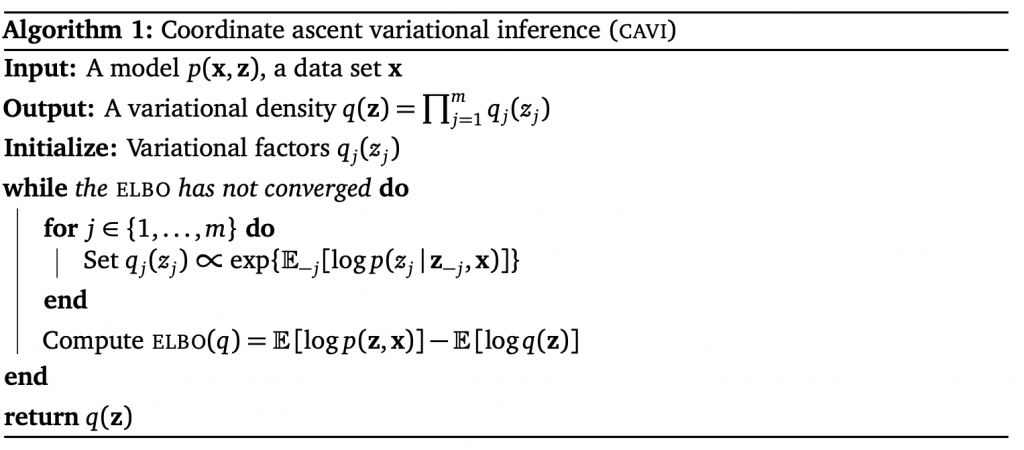
“Set $q_j(z_j) \propto exp\{\mathbb{E}_{-j}[log p(z_j|z_{-j}, x)]\}$ ” may seems hard to understand. It means that setting the variational distribution parameter $\theta_j$ such that $q_j(z_j|\theta_j)$ follows the distribution that is equivalent to $exp\{\mathbb{E}_{-j}[log p(z_j|z_{-j}, x)]\}$ up to a constant. $\mathbb{E}_{-j}$ means that the expectation is taken with regard to a distribution $\prod_{\ell \neq j} q_\ell(z_\ell|\theta_\ell)$ .

What to do after knowing $q(z)=\prod_j q(z_j|\theta_j)$ ?

After the optimization (using CAVI for example), we get the variational distribution $q(z)=\prod_j q(z_j|\theta_j)$ . We can use the estimated $\theta_j$ to analytically derive the mean of $z_j$ or sample $z_j$ from $q(z_j|\theta_j)$ . One thing to note is that there is no restriction on the parametric form of the individual variational distribution. For example, you may define $q(z_j|\theta_j)$ to be an exponential distribution: $q(z_j|\theta_j)=\theta_j e^{-\theta_j z_j}$ . Then, the mean of $z_j$ is $1/\theta_j$ . If $q(z_j|\theta_j)$ is a normal distribution, then $\theta_j$ actually contains two parameters, the normal distribution’s mean and variance. Thus the mean of $z_j$ is simply the mean parameter.

Stochastic Variational Inference

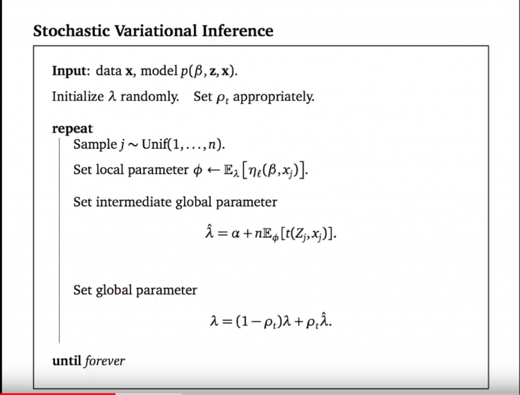
One big disadvantage of CAVI is its scalability. Each update of $\theta_j$ requires full sweep of data to compute the update. Stochastic variational inference (SVI) kicks in because updates of $\theta_j$ using SVI only requires sub-samples of data. The simple idea is to take the gradient of $\nabla_\theta ELBO$ and use it to update $\theta$ . But there is some more detail:

formulas of updates would be very succinct if we assume complete conditionals are in the exponential family: $p(z_j|z_{-j}, x)=h(z_j) exp\{\eta_j(z_{-j},x)^Tz_j - a(\eta_j(z_j, x))\}$ , where $z_j$ is its own sufficient statistics, $h(\cdot)$ , $a(\cdot)$ , and $\eta(\cdot)$ are defined according to the definition of the exponential family [10].
We also categorize latent variables into local variables, and global variables.
the gradient is not simply taken in the Euclidean space of parameters but in the distribution space [11]. In other words, the gradient is transformed in a sensible way such that it is in the steepest descent direction of KL-divergence. Also see [12].

All in all, SVI works as follows [8]:

Reference

[1] https://www.quora.com/Why-and-when-does-mean-field-variational-Bayes-underestimate-variance

[2] ICML 2018 Tutorial Session: Variational Bayes and Beyond: Bayesian Inference for Big Data: https://www.youtube.com/watch?time_continue=2081&v=DYRK0-_K2UU

[3] Variational Inference: A Review for Statisticians

[4] https://towardsdatascience.com/demystifying-kl-divergence-7ebe4317ee68

[5] https://www.zhihu.com/question/31032863

[6] https://blog.csdn.net/aws3217150/article/details/57072827

[7] http://krasserm.github.io/2018/04/03/variational-inference/

[8] NIPS 2016 Tutorial Variational Inference: Foundations and Modern Methods: https://www.youtube.com/watch?v=ogdv_6dbvVQ

[9] https://towardsdatascience.com/making-your-neural-network-say-i-dont-know-bayesian-nns-using-pyro-and-pytorch-b1c24e6ab8cd

[10] https://jwmi.github.io/BMS/chapter3-expfams-and-conjugacy.pdf

[11] https://wiseodd.github.io/techblog/2018/03/14/natural-gradient/

[12] https://czxttkl.com/2019/05/09/gradient-and-natural-gradient-fisher-information-matrix-and-hessian/

[13] https://en.wikipedia.org/wiki/Jensen%27s_inequality

[14] https://github.com/cpark321/uncertainty-deep-learning/blob/master/05.%20Variational%20Inference%20(toy%20example).ipynb