In this post, I’m going to talk about common techniques that enable us to optimize a loss function w.r.t. discrete random variables. I may go off on a tangent on various models (e.g., variational auto-encoder and reinforcement learning) because these techniques come from many different areas so please bear with me.
We start from variational auto encoder (VAE) with continuous latent variables. Then we will look at VAE with discrete latent variables.
VAE
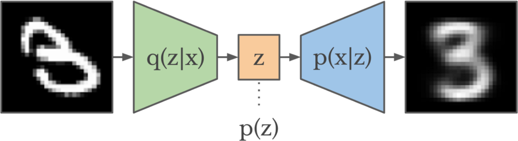
With generative modeling in mind, we suppose every data  is generated by some latent variable
  , which itself is a random variable following certain distribution
  . We’d like to use a parameterized distribution
  to approximate (this is the encoder of VAE). Usually, can be parameterized as a Gaussian distribution:
  . To make and close to each other, we minimize the KL-divergence between them:
![\theta^* = argmin_\theta\; KL\left(q_\theta(z|x) || p(z|x) \right ) \newline= argmin_\theta \; \mathbb{E}_{q_\theta} [log\;q_\theta(z|x)] - \mathbb{E}_{q_\theta} [log\;p(z,x)]+log\;p(x)](https://czxttkl.com/wp-content/ql-cache/quicklatex.com-1acb87f9932eec25d3692cac471a68aa_l3.png "Rendered by QuickLaTeX.com")
In the formula above, ![\mathbb{E}_{q_\theta}[f(z)]](https://czxttkl.com/wp-content/ql-cache/quicklatex.com-5525286df00a53261de88353c9e7658a_l3.png "Rendered by QuickLaTeX.com") means
means  , and
, and  is a constant w.r.t.
  and thus can be omitted. With simple re-arrangement, we can equivalently maximize the so-called ELBO function in order to find
  :
:
![ELBO(\theta) \newline= \mathbb{E}_{q_\theta} [log\;p(z,x)] - \mathbb{E}_{q_\theta} [log\;q_\theta(z|x)]\newline=\mathbb{E}_{q_\theta}[log\;p(x|z)] + \mathbb{E}_{q_\theta}[log\;p(z)] - \mathbb{E}_{q_\theta}[log\;q_\theta(z|x)] \quad\quad p(z) \text{ is the prior of } z \newline= \mathbb{E}_{q_\theta}[log\;p(x|z)] - \mathbb{E}_{q_\theta} [log \frac{q_{\theta}(z|x)}{p(z)}]\newline=\mathbb{E}_{q_\theta}[log\;p(x|z)] - KL\left(q_\theta(z|x) || p(z)\right)](https://czxttkl.com/wp-content/ql-cache/quicklatex.com-8e4bcee52335d51120c9eb549e33fe95_l3.png "Rendered by QuickLaTeX.com")
Practically,  is also fitted by a parameterized function
  (this is the decoder of VAE). So the ultimate objective function we have for fitting a VAE is:
(1) ![\begin{equation*} $argmax_{\theta, \phi} \; \mathbb{E}_{x\sim D} \left[\mathbb{E}_{q_\theta}[log\;p_\phi(x|z)] - KL\left(q_\theta(z|x) || p(z)\right)\right]$\end{equation*}](https://czxttkl.com/wp-content/ql-cache/quicklatex.com-e113a0b22cbcbbbc91b73bf77605c0e6_l3.png "Rendered by QuickLaTeX.com")
We can interpret the objective function in the following ways: ![\mathbb{E}_{q_\theta}[log\;p_\phi(x|z)]](https://czxttkl.com/wp-content/ql-cache/quicklatex.com-cae4aa0a2d5f703241fac19b134f8aef_l3.png "Rendered by QuickLaTeX.com") can be thought as the so-called “reconstruction error”, which encourages the reconstructed be as close to the original as possible.
can be thought as the so-called “reconstruction error”, which encourages the reconstructed be as close to the original as possible.  encourages to be close to the prior of . For more about ELBO and variational inference, please refer to one older post [8].
——————– Update 09/16/2021 ———————
A good post overviewing VAE: https://stats.stackexchange.com/a/315613/80635
Optimize VAE
Optimizing Eq.1 requires additional care. If using stochastic gradient descent, you might want to first sample an from the data distribution  , then sample from , to compute:
(2) 
However, Eq.2 is not the Monte Carlo sampling of the real gradient w.r.t. . This is because  in Eq.1 also depends on the learning parameter . Now we introduce two general ways to optimize Eq.1 [1].
The first method is called score function estimator. From now on, we will ignore the part  . The gradient of Eq.1 w.r.t. can be written as:
(3) ![\begin{align*}&\nabla_\theta \left\{\mathbb{E}_{q_\theta}[log\;p_\phi(x|z)] - KL\left(q_\theta(z|x) || p(z)\right)\right\}\\=&\nabla_\theta \left\{\mathbb{E}_{q_\theta}\left[log\;p_\phi(x, z) - \log q_\theta(z|x)\right] \right\} \quad\quad \text{ rewrite KL divergence} \\ =&\nabla_\theta \; \int q_\theta(z|x) \left[log\;p_\phi(x, z) - \log q_\theta(z|x) \right]dz \\=& \int \left[log\;p_\phi(x, z) - \log q_\theta(z|x) \right]\nabla_\theta q_\theta(z|x) dz + \int q_\theta(z|x) \nabla_\theta \left[log\;p_\phi(x, z) - \log q_\theta(z|x) \right] dz \\=& \mathbb{E}_{q_\theta}\left[ \left(log\;p_\phi(x, z) - \log q_\theta(z|x) \right) \nabla_\theta \log q_\theta(z|x) \right] + \mathbb{E}_{q_\theta}\left[\nabla_\theta \log p_\phi(x, z)\right] + \mathbb{E}_{q_\theta}\left[ \nabla_\theta \log q_\theta(z|x) \right] \\&\text{--- The second term is zero because no }\theta \text{ in } \log p_\phi(x,z) \\&\text{--- The third term being zero is a common trick. See Eqn. 5 in [1]} \\=& \mathbb{E}_{q_\theta}\left[ \left(log\;p_\phi(x, z) - \log q_\theta(z|x) \right) \nabla_\theta \log q_\theta(z|x) \right]\end{align*}](https://czxttkl.com/wp-content/ql-cache/quicklatex.com-ab36fc8bea2fc218505d19ee6e54e94c_l3.png "Rendered by QuickLaTeX.com")
Now we’ve moved the derivative inside the expectation so we can sample from to get Monte Carlo sampling of the gradient.
The second method to optimize Eqn. 1 is called pathwise gradient estimator using the reparameterization trick. We’ve seen the trick used in Soft Actor Critic [9]. Here is how Eqn. 1 can be rewritten with the assumption that  (
( is an independent source of noise):
(4) ![\begin{align*}&\nabla_\theta \left\{\mathbb{E}_{q_\theta}[log\;p_\phi(x|z)] - KL\left(q_\theta(z|x) || p(z)\right)\right\}\\=&\nabla_\theta \left\{\mathbb{E}_{q_\theta}\left[log\;p_\phi(x, z) - \log q_\theta(z|x)\right] \right\} \quad\quad \text{ rewrite KL divergence} \\=&\nabla_\theta \; \int q_\theta(z|x) \left[log\;p_\phi(x, z) - \log q_\theta(z|x) \right]dz \\=&\nabla_\theta \; \int p(\epsilon) \left[log\;p_\phi(x, z) - \log q_\theta(z|x) \right]d\epsilon \quad\quad \\&\text{--- Above uses the property of changing variables in probability density functions.} \\&\text{--- See discussion in [10, 11]} \\=& \int p(\epsilon) \nabla_\theta \left[log\;p_\phi(x, z) - \log q_\theta(z|x) \right]d\epsilon \\=& \int p(\epsilon) \nabla_z \left[log\;p_\phi(x, z) - \log q_\theta(z|x) \right] \nabla_\theta z d\epsilon \\=& \mathbb{E}_{p(\epsilon)} \left[ \nabla_z \left[log\;p_\phi(x, z) - \log q_\theta(z|x) \right] \nabla_\theta f_\theta(x) \right]\end{align*}](https://czxttkl.com/wp-content/ql-cache/quicklatex.com-4fafc4bcaae654c035173052feaa8981_l3.png "Rendered by QuickLaTeX.com")
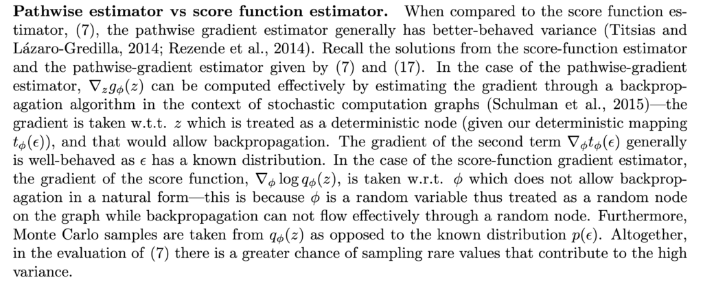
I think [1] summarizes really well that the pathwise estimator generally has lower variance in practice:
In the end, I’d like to share a course which covers more topics on optimization with discrete random variables [6].
Optimize Discrete VAE
The idea of discrete VAE is that the hidden variables are represented as discrete random variables such that it could be better understood by humans as clustering of data. The question remains on how you perform reparameterization trick if is a discrete random variable. The answer is to rely on Gumbel-Softmax trick [12].
Suppose a discrete random variable has  classes with class probability
  , which can be parameterized by a neural network consuming the raw data. There are several steps to perform the Gumbel-Softmax trick. First, is represented as a one-hot encoding vector. The active component would be the one with the highest following quantity:
(5) ![\begin{align*}\arg\max_i \left[ g_i + log \pi_i \right]\end{align*}](https://czxttkl.com/wp-content/ql-cache/quicklatex.com-e0bca8c8b12be82c3fe266e5e8121352_l3.png "Rendered by QuickLaTeX.com")
The beauty of Eqn.5 is that this is equivalent to draw a sample based on the probability distribution
.
Second, the one-hot encoding vector is relaxed to a continuous vector  , with each component as:
(6) 
where
 are i.i.d. samples drawn from
  distribution, and
  will be annealed through the training such that
  will be closer and closer to a one-hot encoding vector.
Finally, depending on specific problems, we will forward as some differentiable quantity to downstream models (discussed in Section 2.2. in [12]). If the problem is about learning hidden representations, we can have fully connected layers on top of the whole . If the problem would require sampling discrete actions as in reinforcement learning, in forward pass we would need to sample an action by  on while in backward pass we would use Straight-Through operator by approximating
  .
.
Here is an example of Gumbel-Softmax trick-based discrete VAE, which I adapted from [13]. In the code, we create 30 10-category random variables as the hidden representation . As a result, becomes a 300-dim continuous vector during the training. While in testing (where we create images in data/sample_), we randomly create 30 one-hot encoding vectors of dim 10 as the hidden representation, and ask the decoder to generate images for us.
An earlier attempt to train discrete VAE can be seen in [5] and [3]. It uses embedding table look up + straight through to train such discrete VAE models.
References
[1] Lecture Notes. Part III: Black-Box Variational Inference
[2] http://edwardlib.org/tutorials/klqp
[3] Reproducing Neural Discrete Representation Learning
[4] https://github.com/ritheshkumar95/pytorch-vqvae
[5] Neural Discrete Representation Learning
[6] https://duvenaud.github.io/learn-discrete/
[7] Discrete Variational Autoencoders
[8] https://czxttkl.com/2019/05/04/stochastic-variational-inference/