In this post, I am going to share my understanding in Bayesian Optimization. Bayesian Optimization is closely related Gaussian Process, a probabilistic model explained in details in a textbook called “Gaussian Processes for Machine Learning” [1]. In the following, “p. ” will refer to a specific page in [1] where the content comes from.
First, let’s dive into the detail of Gaussian Process.
We need to have a new thinking model in our mind: think any function $latex f(x)$ as a very long vector, each entry in the vector specifying the function value $latex f(x)$ at a particular input $latex x$ (p. 2). Of course, in theory, this vector will be arbitrarily, infinitely long because we can measure $latex f(x)$ at arbitrarily scaled precision. Let’s make it clear that $latex x$ is the input of $latex f(x)$ and it has $latex d$ dimension: $latex x \in \mathbb{R}^d$. Usually, we let $latex x$ be a column vector.
One step further, we need to think the function vector as a vector of random variables. Each entry of the vector is a random variable, meaning that there is a probability distribution for every $latex f(x)$ at a specific $latex x$. Since they are all random variables, any finite number of the entries can be selected to form a joint probability distribution.
Let $latex X \in \mathbb{R}^{n \times d}$ be the aggregation matrix of $latex x$ corresponding to the picked entries. Let $latex f=\{f(X_{i})\}_{i=1}^n$, a vector of $latex f(x)$ at different $latex x$ in $latex X$. If we assume $latex f(x)$ follows Gaussian Process (p. 13), then the joint probability distribution of $latex f$ (induced by any $latex X$) will be a Gaussian distribution:
$latex f \sim \mathcal{N}(m(X), K(X, K)),&s=2$
where $latex m(X) \in \mathbb{R}^n$ is a mean function vector whose each entry is defined as $latex m(x)=\mathbb{E}[f(x)]$; and $latex K(X, X) \in \mathbb{R}^{n \times n}$ is the covariance matrix of the Gaussian distribution. The entry on $latex p$ row, $latex q$ column, $latex K_{pq}(X, X)$, is defined as a covariance function between $latex x_p$ and $latex x_q$: $latex k(x_p, x_q)=\mathbb{E}[(f(x_p)-m(x_p))(f(x_q)-m(x_q))]$.
For such $latex f(x)$ following Gaussian Process, we can write as: $latex f(x) \sim \mathcal{GP}(m(x), k(x, x’))$, reading as “$latex f(x)$ follows a Gaussian Process governed by a mean function $latex m(x)$ and a covariance function $latex k(x,x’)$”.
Let’s now look at a Bayesian linear regression model $latex f(x)=\phi(x)^T w$ with $latex \phi(x)$ as a feature transformation function to transform $latex x$ into a high-dimension space and a prior distribution $latex w \sim \mathcal{N}(0, \Sigma_p)$.
For any $latex x$, $latex \mathbb{E}[f(x)] = \phi(x)^T \mathbb{E}[w] = 0$. For any $latex x$ and $latex x’$, $latex \mathbb{E}[(f(x)-m(x))(f(x’)-m(x’))] = \phi(x)^T \mathbb{E}[w w^T]\phi(x’) = \phi(x)^T \Sigma_p \phi(x’)$ (p. 14). Actually, for any finite number of inputs $latex x_1, x_2, \cdots, x_n$, the function values $latex f(x_1), f(x_2), \cdots, f(x_n)$ forms a joint Gaussian distribution with zero means and convariance given as $latex k(x, x’)=\phi(x)^T \Sigma_p \phi(x’)$: $latex f \sim \mathcal{N}(0, K(X, X))$. Therefore, we can say $latex f(x)$ in the Bayesian linear regression model follows a Gaussian Process.
If we set $latex k(x, x’)=\phi(x)^T \Sigma_p \phi(x’) = exp(-\frac{1}{2}|x – x’|^2)$, then this corresponds $latex \phi(x)$ to transform $latex x$ into an infinite feature space. We call this covariance function squared exponential (SE) or radial basis function (RBF). Please review [2] for kernel methods introduced in SVM. There of course exist many other covariance functions. Different covariance functions will govern the shape of the joint Gaussian distribution of $latex f$ (and also the conditional distribution of new $latex f$ given observations, which we will talk next). From now on, we will assume we use SE as the covariance function.
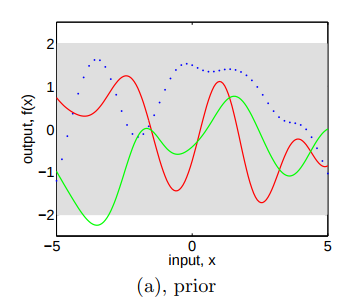
Since we have $latex f \sim \mathcal{N}(0, K(X, X))$ as the joint distribution for any finite number of $latex x$, we can draw multivariate samples from the joint distribution. Figure 2.2 (a) (p.15) shows three drawn samples: first, we prepare a series of equidistant $latex x$, say, -5.0, -4.9, -4.8, … 4.8, 4.9, 5.0, which can be aggregated to a matrix $latex X$; then, we draw $latex f(x)$ according to $latex f \sim \mathcal{N}(0, K(X, X))$. By connecting the generated points $latex (x, f(x))$ we get three functions (the red line, the green line, or the dotted blue line). The gray area represents the pointwise mean plus and minus two times the standard deviation for each input value. Because we know $latex m(x)=0$ and $latex k(x,x’)=1$ for all $latex x$, the gray area is actually a rectangle between 2 and -2.
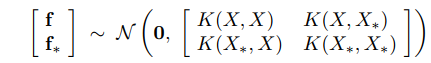
So far we are only dealing with a Gaussian Process prior because we have not observed any data therefore no more information can be utilized. The most interesting part comes as we have some (for now, we assume noiseless) observations $latex \{(x_i, f_i)|i=1,\cdots,n\}$ and we want to extract any insight to make more accurate guess about new the function values at new $latex x$. We will use $latex f$ to denote the observation outputs, and $latex f_*$ for new test outputs. We will use $latex X_*$ to denote the aggregated matrix of test $latex x$. Because $latex f(x)$ follows a Gaussian Process, $latex [f, f_*]$ still forms a joint Gaussian distribution (p.15):
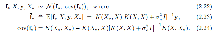
The most important part is that we want to infer future $latex f_*$ based on observed $latex f$. Therefore, we shouldn’t merely look at the joint distribution but instead should focus on the conditional distribution $latex f_*|X_*, X, f$, which can also be called the posterior distribution. It turns out that the posterior distribution is still a Gaussian distribution (p. 16):
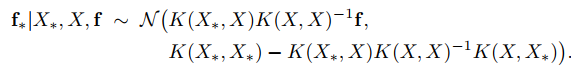
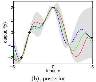
Figure 2.2 (b) (p.15) shows three randomly drawn functions obtained in a similar manner as in Figure 2.2 (a) based on the posterior distribution: first, we prepare a series of equidistant $latex x_*$, say, -5.0, -4.9, -4.8, … 4.8, 4.9, 5.0, which can be aggregated to a matrix $latex X_*$; then, we draw $latex f_*$ according to $latex f_*|X_*,X,f$. By connecting the generated points $latex (x_*, f_*)$ we get three functions (the red line, the green line, or the blue line). Note that, the gray area is no longer constant: in the area close to observations, the pointwise standard deviation is small; it is larger in less observation-dense areas indicating less confidence:
In the following chapters of [1], it continues to introduce the situation when our observations are not noise-free. In this situation, the posterior distribution becomes (p. 16):
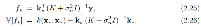
In the case that there is only one test point $latex x_*$, we write $latex k(x_*)=k_*$ to denote the vector of covariances between the test point and the $latex n$ training points and we have:
So far we’ve derived the posterior distribution from a function space view. What is interesting is that the same posterior distribution can be obtained from a pure probabilistic way (i.e., weight space view), a way we are more familiar with, without thinking functions in a function space.
It starts from Bayesian Theorem:
$latex p(w|y,X) = \frac{p(y|X,w)p(w)}{p(y|X)} \propto p(y|X,w) p(w) &s=2$
In a Bayesian linear model, we assume $latex y=f(x) + \epsilon$, $latex \epsilon \sim \mathcal{N}(0, \sigma_n^2)$ and $latex w \sim \mathcal{N}(0, \Sigma_p)$. Therefore,
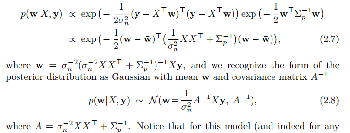
The posterior distribution given observation $latex X$, $latex y$ and new $latex x_*$ becomes (p. 11):
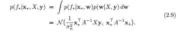
To empower a linear model, we can use a feature transformation $latex \phi(x)$ to transform $latex x$ into a high-dimensional space and apply the linear model in that space: $latex f(x) = \phi(x)^T w$. The posterior distribution changes accordingly (p. 12):
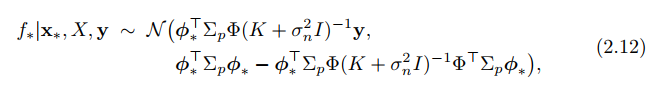
In Eqn. 2.12, the transformed features only enter in the form of $latex \phi_*^T\Sigma_p\phi$, $latex \phi_*^T\Sigma_p\phi_*$ and $latex \phi^T\Sigma_p\phi$. This can be again thought as some form of kernel: $latex k(x,x’)=\phi(x)^T\Sigma_p\phi(x’)$. Therefore, we arrive at the same posterior distribution as in Eqn. 2.22~2.24.
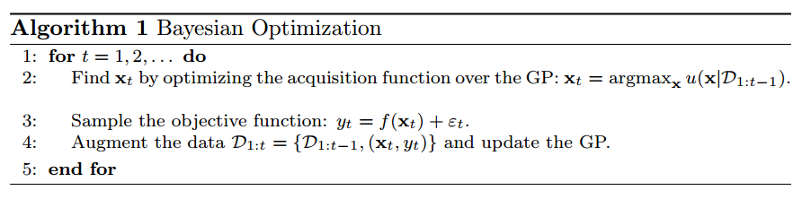
We finished introducing Gaussian Process. Now, we introduce Bayesian Optimization. Bayesian Optimization is mostly used for black-box optimization:
$latex max_x f(x), &s=2$
where the objective function $latex f(x)$ is assumed to have no known analytic expression and expensive to evaluate. The idea is to iteratively make guess about next promising observation based on existing observations until the (approximated) optimum is found [3]. The guess will be based on a constructed acquisition function, which has some closed form and is much cheaper to evaluate than the original objective function. People have proposed many forms of acquisition function. One thing for sure is that they all rely on the posterior distribution $latex f_*|X_*, X, f$. The link between Gaussian Process and Bayesian Optimization is that Bayesian Optimization assumes the black-box function to be maximized follows Gaussian Process thus the posterior distribution $latex f_*|X_*, X, f$ will follow a Gaussian distribution we know how to express analytically.
Intuitively, a good acquisition function should not only favor the area where the posterior mean is high (so it can exploit learned information), but also favor the area with much uncertainly (so that further exploration can be performed). One popular of such acquisition function is called Expected Improvement (EI):
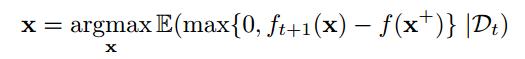
where $latex x^+=argmax_{x_i \in x_{1:t}} f(x_i)$. Interpreted this expression in English, it speaks that we want to find the next $latex x$ that has the largest expected improvement of the best $latex x^+$ so far. If we are unsure about $latex f(x)$ at $latex x$, $latex EI(x)$ will also be large.
If we set the pointwise mean and standard deviation of the posterior distribution of $latex f_{t+1}(x)$ as $latex \mu(x)=\bar{f}_*$ and $latex \sigma^2(x)= \mathbb{V}[f_*]$ [See equation 2.25 and 2.26 (p.17)], and if we set a random variable $latex I=\mathbb{E}[max\{0, f_{t+1}(x)-f(x^+)\}]$, we will have:
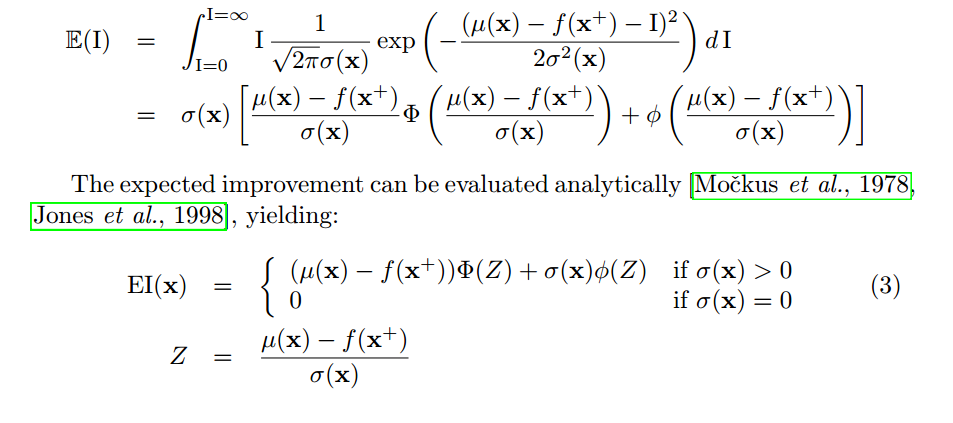

We’ve known how to compute $latex EI(x)$, the acquisition function. The only remaining question is now how to sample next $latex x$. This remains a practical problem that I will investigate the future. But the whole idea of Bayesian Optimization has been clear now.
Reference
[1] http://www.gaussianprocess.org/gpml/
[2] https://czxttkl.com/?p=3114
[4] Bayesian Optimization with Inequality Constraints
Two informal posts:
[] https://arimo.com/data-science/2016/bayesian-optimization-hyperparameter-tuning/
[] https://thuijskens.github.io/2016/12/29/bayesian-optimisation/