Revisit Gaussian kernel

This post is mainly about Gaussian kernel (aka radial basis function kernel), a commonly used technique in machine learning. We’ve touched the concept of Gaussian kernel in [1] and [2] but with less details.

Definition of Gaussian Kernel

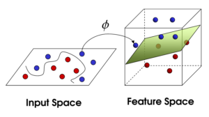
The intuitive understanding of a kernel is that it maps points in a data space, where those points may be difficult to be classified, to a higher dimensional space, where the corresponding mapped points are easier to be separable.

Gaussian kernel is defined as:

$K(\mathbf{x}, \mathbf{y})=exp\left(-\frac{\|\mathbf{x}-\mathbf{y}\|^2}{2\sigma^2}\right),$

where $\mathbf{x}$ and $\mathbf{y}$ are two arbitrary points in the data space, $\sigma$ is a hyperparameter of the Gaussian kernel that controls the sensitivity of difference when $\mathbf{x}$ and $\mathbf{y}$ are different. Imagine $\sigma$ goes to infinity, then no matter how different $\mathbf{x}$ and $\mathbf{y}$ are, $K(\mathbf{x}, \mathbf{y})$ will be 1. The formula of Gaussian kernel is identical to the PDF of a normal distribution.

$K(\mathbf{x}, \mathbf{y})$ can be understood as the distance between the corresponding points of $\mathbf{x}$ and $\mathbf{y}$ in the mapped higher dimensional space (denoted as $\phi(\mathbf{x})$ and $\phi(\mathbf{y})$ ). The higher dimensional space is actually an infinite dimensional space, and the distance is measured by the dot product. That is, $K(\mathbf{x}, \mathbf{y}) = <\phi(\mathbf{x}), \phi(\mathbf{y})>$ .

So what is $\phi(\mathbf{x})$ then? According to ([3] page 11), we have:

Application of Gaussian Kernels

Using Gaussian kernels, we can design classification/regression algorithms and their ideas would be similar to nearest neighbor algorithms. Here is how [4]. Suppose we have $N$ data points $\mathbf{x}_1, \cdots, \mathbf{x}_N$ with their labels $y_1, \cdots, y_N$ . Each of the $N$ data points will contribute some information $w_n$ to the prediction of a new data point $h(\mathbf{x})$ .

Intuitively, those $\mathbf{x}_n$ that are close to $\mathbf{x}$ should contribute more information; those $\mathbf{x}_n$ that are far away from $\mathbf{x}$ should contribute less information. Therefore, we use a Gaussian kernel $K(\mathbf{x}, \mathbf{x}_n)=exp\left(-\gamma \|\mathbf{x}-\mathbf{x}_n\|^2\right)$ to denote the degree of $w_n$ that $\mathbf{x}_n$ should contribute to $h(\mathbf{x})$ . This screenshot comes from [4], where $\gamma = \frac{1}{2\sigma^2}$

The way to learn $w_n$ is that we want $h(\mathbf{x})=0 \text{ for } \mathbf{x}=\mathbf{x}_1, \cdots, \mathbf{x}_N$ . Therefore, we can solve the following matrix-vector equation to obtain $\mathbf{w}$ :

Once we have $\mathbf{w}$ , we have full information of our regression/classification model $h(\mathbf{x})$ , and we can use it to make prediction to unseen data.

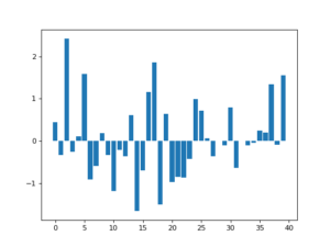
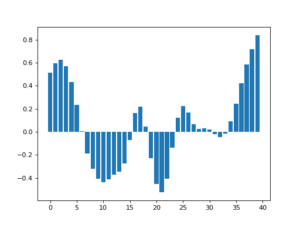
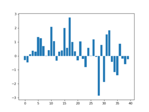
We can use Gaussian kernel to perform smoothing. In [11], the author detailed some examples of applying Gaussian kernel for smoothing. In the example below, the authors generated some noisy data in 1D array (left). By applying a Gaussian kernel, that is averaging the values mostly from the neighborhood, we get a much smoother data distribution (right).

Magically, applying a correct Gaussian kernel can recover from noisy data that seems random. Below, we can see that a clean data distribution (up left), after added with noise (up right), can be recovered mostly if the Gaussian kernel “matches” certain characteristics of the noise (bottom).

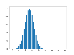
Another application of Gaussian kernels is to perform kernel density estimation [5]. It is a technique to depict a smooth probability distribution from finite data samples. The smoothness of the probability distribution is determined by the hyperparameter $\sigma$ . When $\sigma$ is small, the distribution will look like histograms because the kernel will average data on near neighbors. Larger $\sigma$ will have wider focus on data.

Convolution and Fourier Transform

Gaussian kernels can be used in the setting of convolution and Fourier transform. We first quickly review what convolution and Fourier transform are and their relationships.

A convolution of two functions is defined as:

$f(t)=(g*h)(t)=\int^\infty_{-\infty}g(\tau)h(t-\tau)d\tau$

For a function that is on the time domain $f(t)$ , its frequency domain function $\hat{f}(\xi)$ is defined as:

$\hat{f}(\xi)=\int^{\infty}_{-\infty}f(t)e^{-2\pi i t \xi} dt$

And the inverse Fourier transform is defined as:

$f(t)=\int^\infty_{-\infty}\hat{f}(\xi)e^{2\pi i t \xi} d\xi$

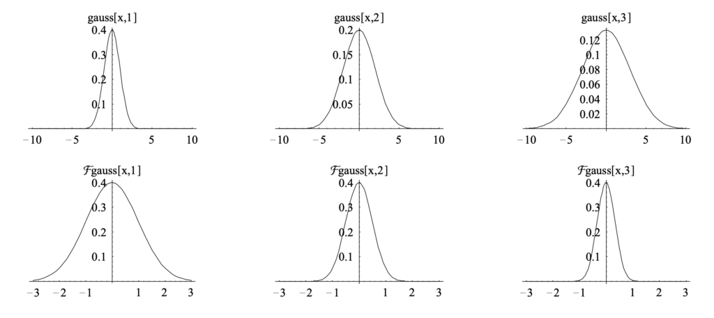
If $f(t)$ itself is a Gaussian function, then $\hat{f}(\xi)$ would also be a Gaussian function but with different shapes. The more spread $f(t)$ is, the sharper $\hat{f}(\xi)$ is [9]. This means, a spread $f(t)$ changes slowly so it has less high-frequency components.

Now let’s prove the convolution theorem, which states that the Fourier transform of the convolution of two functions is equal to the product of the Fourier transform of each function. The proof comes from the last page of [10]:

Suppose we have $f(t)=(g*h)(t)=\int^\infty_{-\infty}g(\tau)h(t-\tau)d\tau$ , and suppose $\hat{f}(\xi)$ , $\hat{g}(\xi)$ , and $\hat{h}(\xi)$ are the corresponding Fourier transformed functions. From the inverse Fourier transform we have $g(t)=\int^\infty_{-\infty} \hat{g}(\xi) 2^{\pi i t \xi}d\xi$ and $h(t)=\int^\infty_{-\infty} \hat{h}(\xi) 2^{\pi i t \xi}d\xi$ .

By the definition of convolution:

$(g*h)(t)=\int^\infty_{-\infty}g(\tau)h(t-\tau)d\tau \newline=\int^\infty_{-\infty} g(\tau)\left[\int^\infty_{-\infty} \hat{h}(\xi) 2^{\pi i (t-\tau) \xi}d\xi\right]d\tau \newline=\int^\infty_{-\infty} \hat{h}(\xi) \left[\int^\infty_{-\infty} g(\tau) 2^{\pi i (t-\tau) \xi}d\xi\right]d\tau \quad \quad \text{swap } g(\tau)\text{ and }\hat{h}(\xi)\newline=\int^\infty_{-\infty} \hat{h}(\xi) \left[\int^\infty_{-\infty} g(\tau) 2^{-\pi i \tau \xi} d\tau\right] 2^{\pi i t \xi} d\xi\newline=\int^\infty_{-\infty} \hat{h}(\xi) \hat{g}(\xi) 2^{\pi i t \xi} d\xi \newline = IFT\left[\hat{h}(\xi) \hat{g}(\xi)\right] \quad\quad Q.E.D.$

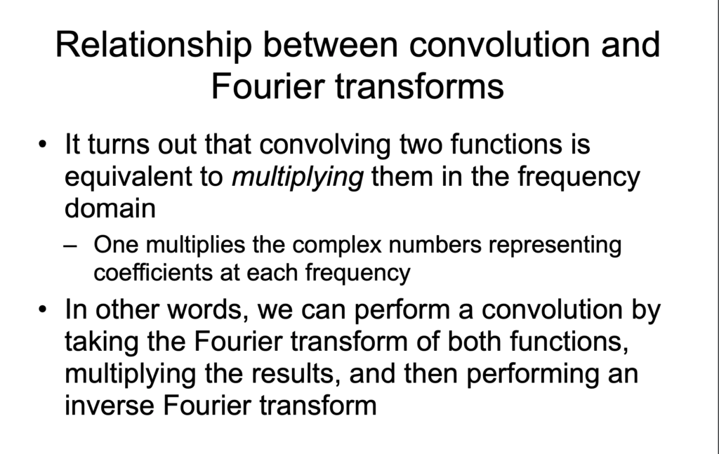
I think [6] summarizes well the relationship between convolution and Fourier Transform [7].

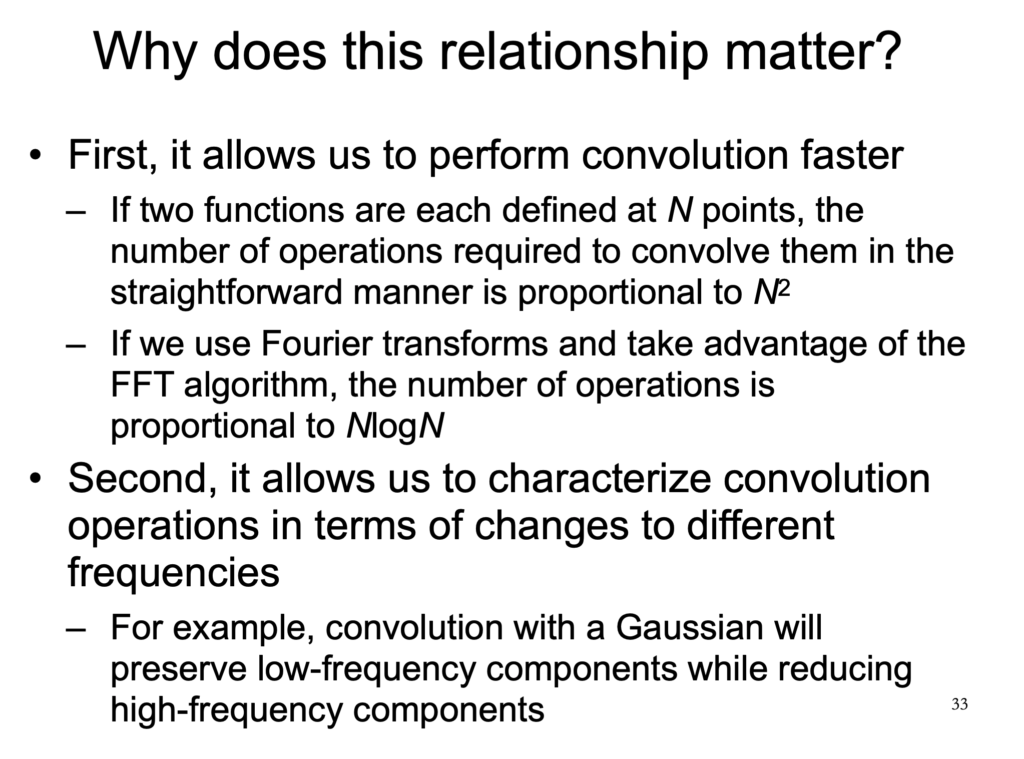
Now let’s understand the last sentence from the last slide: convolution with a Gaussian will preserve low-frequency components while reducing high-frequency components.

Suppose we have a rectangle function $h(t) =\sqcap(t/2)$ with width 2 and height 1.
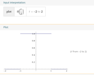We know that its fourier transform is (https://www.wolframalpha.com/input/?i=+rect%28t%2F2%29+from+-2+to+2):

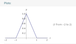
After applying Gaussian kernel smoothing (e.g., $g(t)=gaussian(0, 1)$ , as we introduced in the application section, we probably get a smoother function roughly like a triangle function $f(t)=(g*h)(t)=\Lambda(t)$ (https://www.wolframalpha.com/input/?i=triangle%28t%29):

$\Lambda(t)$ ‘s fourier transform is (https://www.wolframalpha.com/input/?i=fourier+transform+%28triangle%28t%29%29):

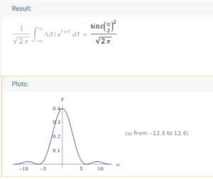
Apparently, we can see that the high frequency components of $\Lambda(t)$ is much smaller than those of $\sqcap(t/2)$ .

From the point of the convolution theorem to understand this phenomenon, the fourier transform of $(g*h)(t)$ is equal to $\hat{g}(\xi) \hat{h}(\xi)$ . We know that $\hat{h}(\xi)$ is a $sinc$ function and $\hat{g}(\xi)$ is a gaussian function, therefore the high frequency components of $\hat{g}(\xi)\hat{h}(\xi)$ would be attenuated.

References

[1] https://czxttkl.com/2018/01/20/my-understanding-in-bayesian-optimization/
[2] https://czxttkl.com/2017/12/28/revisit-support-vector-machine/
[3] https://www.csie.ntu.edu.tw/~cjlin/talks/kuleuven_svm.pdf
[4] https://www.youtube.com/watch?v=O8CfrnOPtLc
[5] http://www.surajrampure.com/resources/ds100/KDE.html
[6] https://web.stanford.edu/class/cs279/lectures/lecture9.pdf
[7] https://czxttkl.com/2018/10/07/eulers-formula/
[8] https://en.wikipedia.org/wiki/Fourier_transform#Other_conventions
[9] http://pages.stat.wisc.edu/~mchung/teaching/MIA/reading/diffusion.gaussian.kernel.pdf.pdf
[10] http://ugastro.berkeley.edu/infrared09/PDF-2009/convolution2.pdf
[11] https://matthew-brett.github.io/teaching/smoothing_intro.html