We’ve covered Fourier Transform in [1] and [2] while we use only examples of 1D. In this post we are going to see what 2D Fourier Transform looks like.
First, we look at a 2D image with one direction sinusoid waves (left) and its Fourier Transform (right).
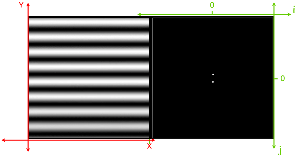
I added coordinates to help you understand the illustration. Let’s assume the  -axis in the image corresponds to
  -axis in frequency domain;
  -axis in the image corresponds to
  -axis in the frequency domain. Because there is never fluctuation along the -axis, there should only be
  frequency. However, along the -axis there is regular sinusoid change, therefore there should be
  frequency. As a combination, we see two dots (two dirac delta functions) on the line .
To reinforce our understanding, let’s look at three more pictures. The first two have vertical bars with different spatial frequencies. As you might guess, the first picture with sparser bars have a smaller frequency than the second picture. Their frequencies are only on the line  because there is no signal variation on the -axis.
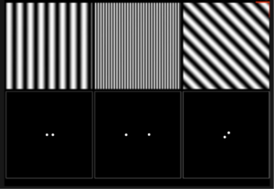
The third picture is generated by  (https://www.wolframalpha.com/input/?i=+plot+sin%28x%2By%29). And it has regular variations of waves along both the and -axis. Thus, we see the two white dots in the frequency domains are on a diagonal.
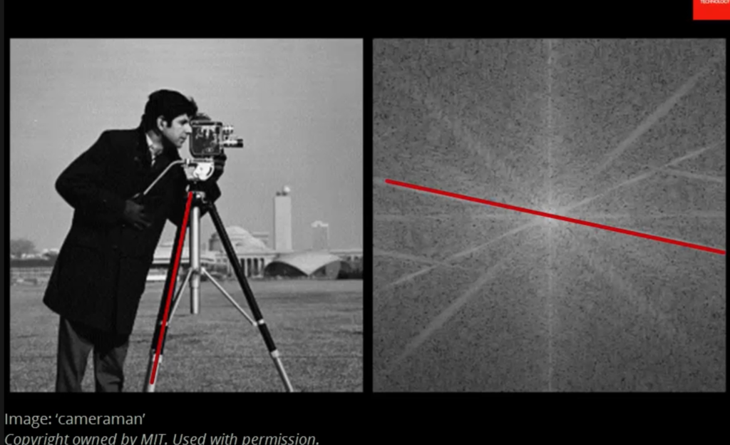
Next, we examine a real-world photo, a famous picture titled “cameraman”. We mark one leg of the tripod in th image and its corresponding frequency band. This leg is almost perpendicular to the -axis. Therefore, it introduces high-frequency variation (sharp edges) along the direction of -axis. Meanwhile it introduces less variation on the direction of -axis. On the frequency domain, you can see the corresponding line has a slope more towards the -axis than the -axis.
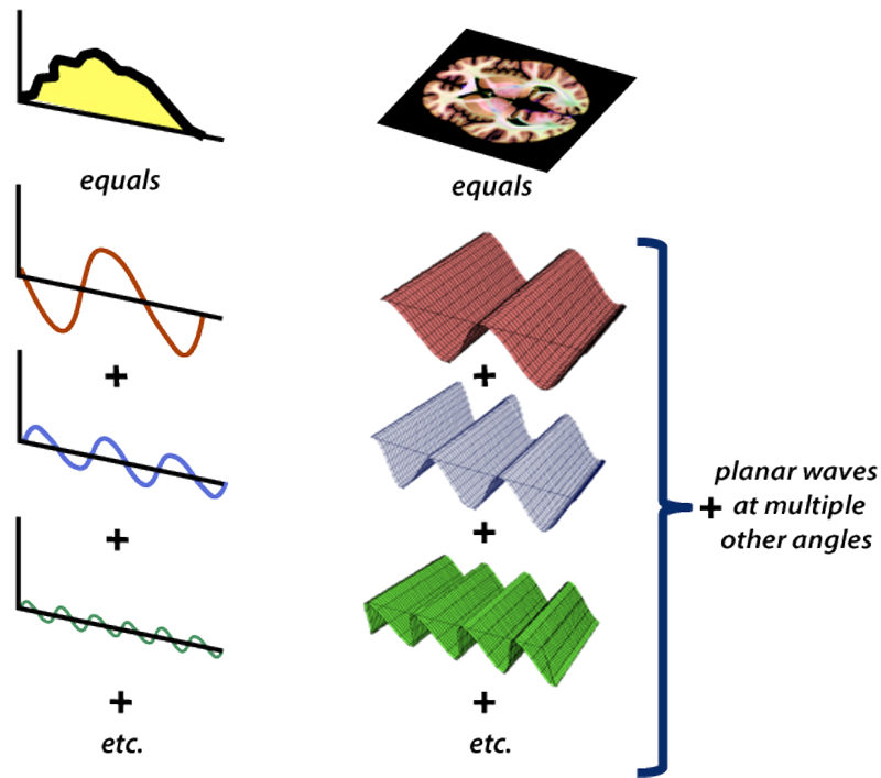
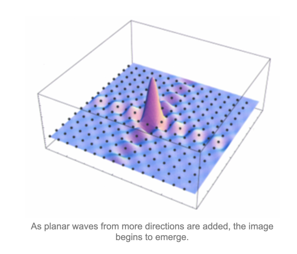
At last, let’s revisit how images are constituted. In essence, images are formed by 2D waves, just like 1D functions are formed by 1D waves:


References
[1] https://czxttkl.com/2018/10/07/eulers-formula/
[2] https://czxttkl.com/2020/04/27/revisit-gaussian-kernel/
Image examples come from:
[3] https://www.youtube.com/watch?v=YYGltoYEmKo
[4] https://homepages.inf.ed.ac.uk/rbf/HIPR2/fourier.htm
[5] https://www.youtube.com/watch?v=gwaYwRwY6PU
A website that is helpful in visualizing 2d function: