This post reviews the key knowledgement about support vector machine (SVM). The post is pretty much based on a series of the lectures [1].
Suppose we have data  , where each point is a
  -dimensional data point
  associated with label
  .
.
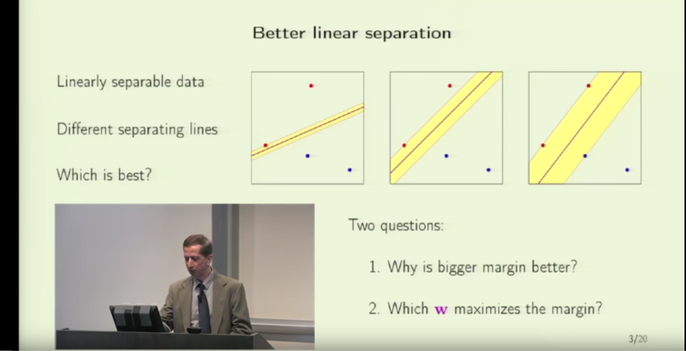
The very initial SVM is to come up with a plane  such that data points can be perfectly linearly divided according to their labels. For a linearly separable dataset, there can exist infinite such plane. However, the “best” one, intuitively, should have the largest margins from all the closest points to it. Here, “margin” means the distance from a point to a plane. As an example below, the best separating plane is supposed to be the rightmost one.
For a data point  , the way to calculate its margin (i.e., its distance to the plane
  , is to pick a point
  on the plane and then project
  onto
onto  :
:
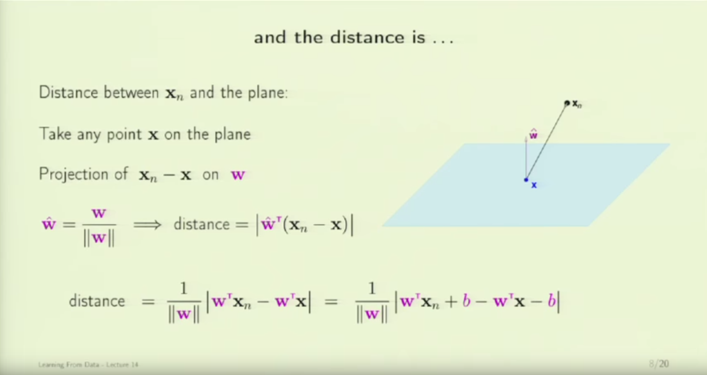
Since any point on the plane satisfies that , we can simplify the distance formula:

(From an intuitive perspective, the vector is perpendicular to the plane  . Therefore the distance from to the hyperplane is to find the projection of onto the direction .)
This is the margin for any data point . However, remember that the ultimate goal is to maximize the margin of the data point, the data point which is the closest to the separating plane. One can write the objective function like this:

A problem arises here. Even for the same plane, there can be infinite sets of  corresponding to it, all with different scales. For example, the plane
  with
with  is the same plane as the plane
  with
with  . Therefore, we need to pre-define a scale.
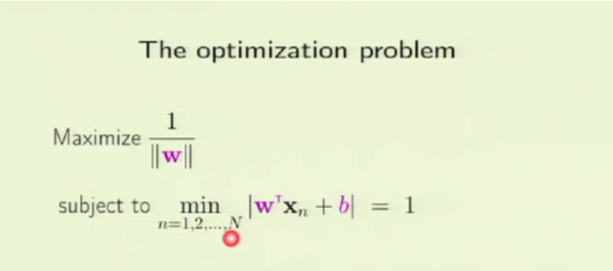
We propose a normalization standard: normalize and  such that the closest data point to the plane, , has:
  . Therefore, the distance from the closest data point to the plane becomes
  . After this, the objective function becomes easier:
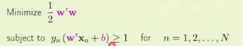
Note that for any data point ,  . The constraints
  can be re-written as
  . Moreover, instead of maximizing , we can minimize
  equivalently. Therefore, the objective function now becomes:
We are sure that for all the constraints, there must be at least one constraint where the equality holds (i.e., for some data point ,  ). That is the data point which is the closest to the plane. If all the constraints only have the inequality hold (i.e.,
  ), would not be minimized: we can always scale down a little bit such that
  decreases until some constraint hits the equality.
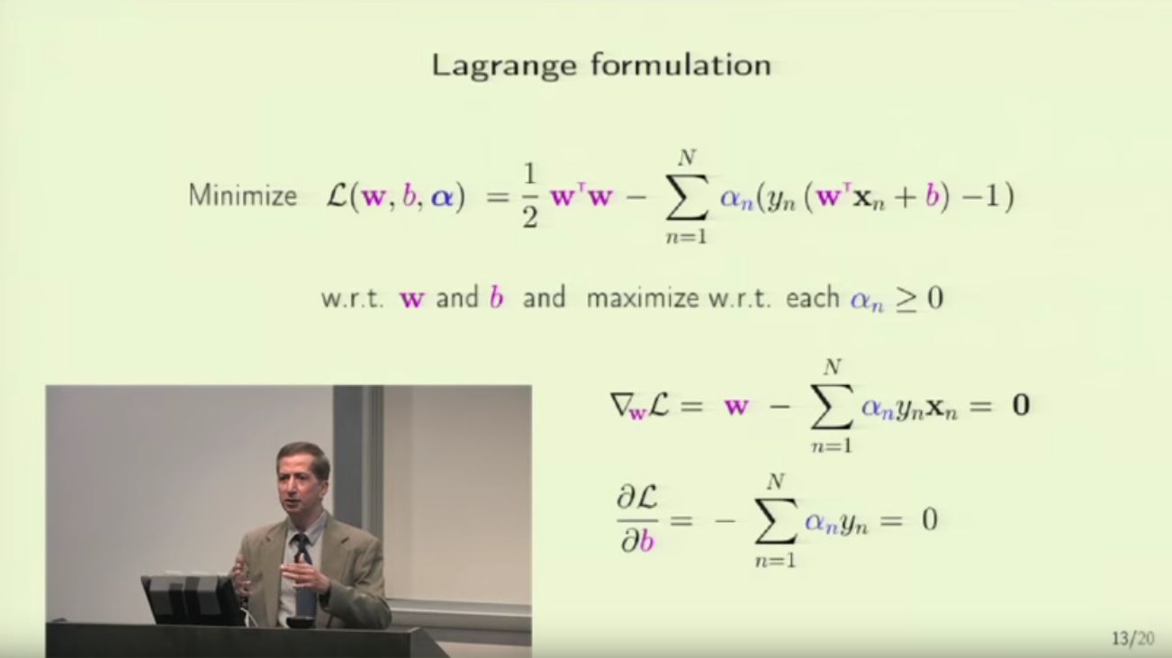
The objective function is a constrained optimization problem with affine inequality constraints. An overview of using Lagrange/KKT to do optimization can be found in my previous post [2]. Basically, the way to optimize this objective function is to use Lagrange multiplier and KKT condition.
From [2], we know that KKT condition is usually a necessary condition in a constrained optimization problem. However, when the optimization problem is convex (in our case ) and Slater’s condition holds (in our case, we only have linear constraints  ), KKT condition becomes a sufficient and necessary condition for finding the optimal solution
  . will be the saddle point of the Lagrange multiplier augmented loss function . Regarding why we can apply Lagrange multiplier + KKT condition to optimize the objective function, please refer to other materials also, since this is the part I am less confident about: (Section 3.2 in [4], answer in [5], slides in [6], Section 5.2.3 in [7]).
The optimization process is as follows. We first write the Lagranger formulation and take the derivatives of the Lagranger formulation w.r.t. and . Setting the derivatives to 0 we can find the relationship between  (the Lagranger multipler),
  , and (data).
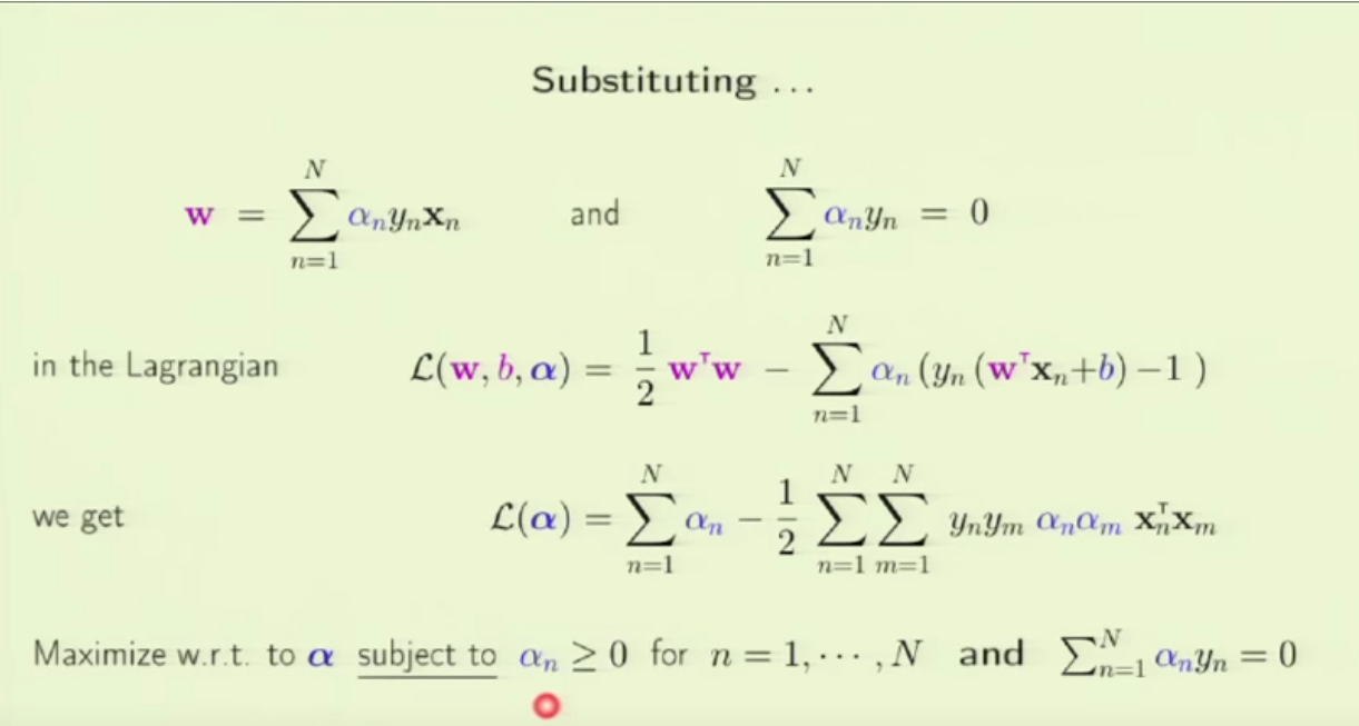
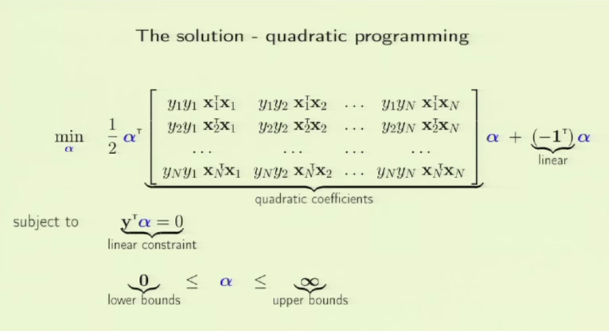
We can eventually formulate the problem as a quadratic programming problem (w.r.t. ) and then hand it to a quadratic programming package to solve it. We are expected to receive the vector as results, which then we will use to obtain .
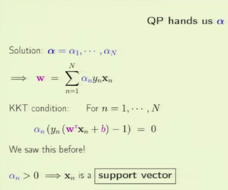
Then, the parameter can be obtained by picking a support vector and solve by  .
.
Until this point, a new problem arises: we have been only dealing with perfectly linearly separable problems. How can we apply SVM in non-linear problems?
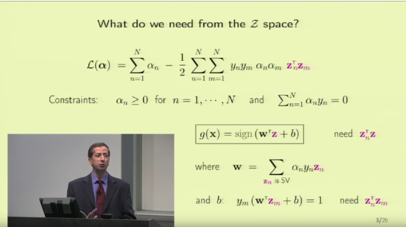
The first solution is kernel trick. Our objective function sending to quadratic programming is  , which only requires we know the inner product between any and
  . Suppose in the original form of raw data,
  are low-dimensional data points that are not linearly separable. However, if they are mapped to a higher dimension as
  , they can be separable. On that high dimension space, we can apply the linear separable SVM version on the data points to find a hyperplance and support vectors. That only requires we know the inner product of
  and
and  .
.
We don’t even need to know the exact formula of the mapping function from  : even a black-box mapping function is ok, as long as we can calculate the inner product of any and corresponding to and . This “inner product” value function is called kernel:
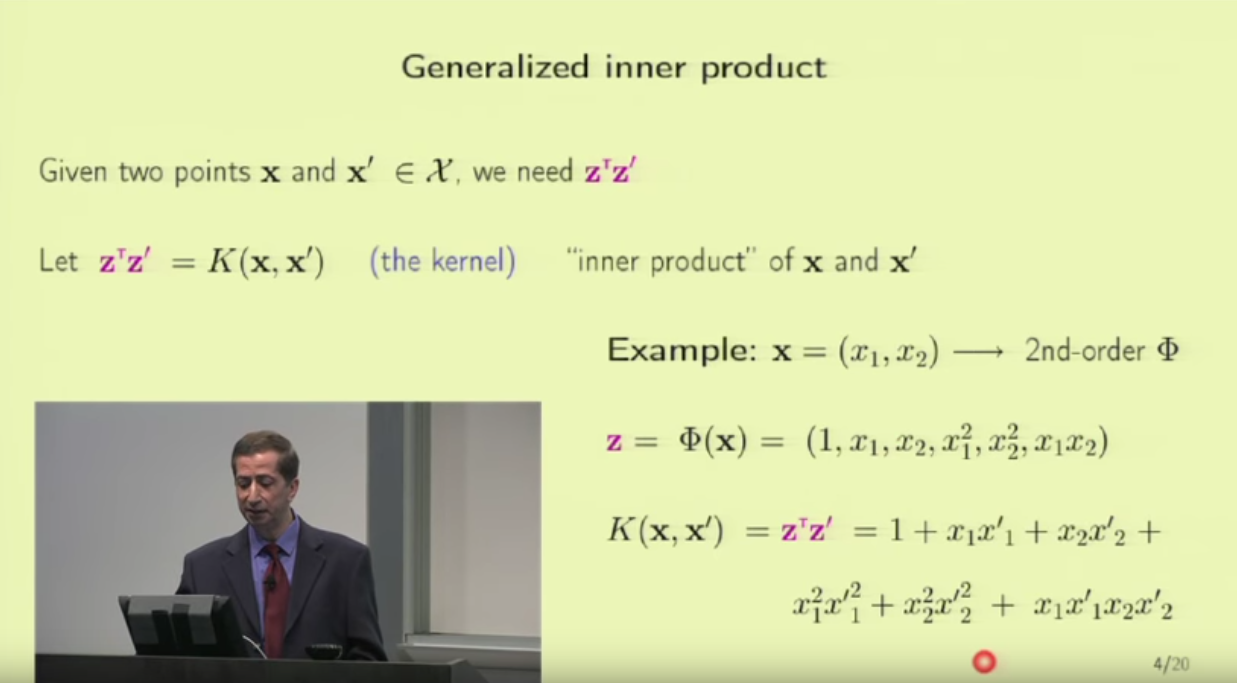
Kernel functions can have many forms. For example, polynomial kernel:  and Radial Basis Function kernel:
  . There is a math property called “Mercer’s condition” that an be used to verify whether a function is a valid kernel function. But this is out of the scope of this post.
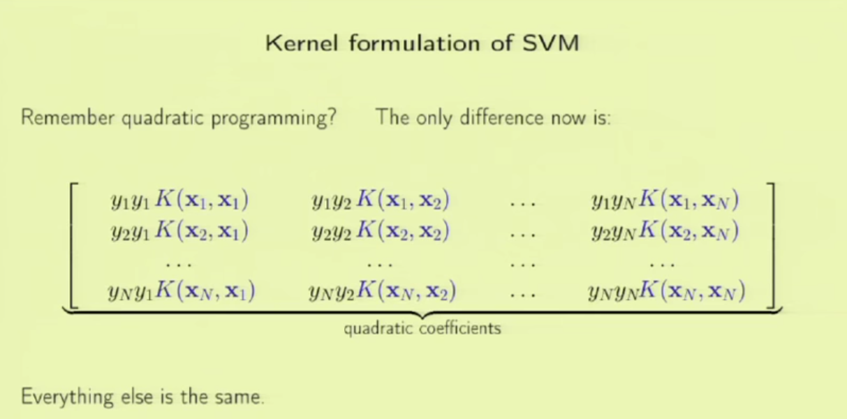
After we use kernel, the optimization of SVM stays the same except that the coefficient matrix of quadratic programming now becomes:
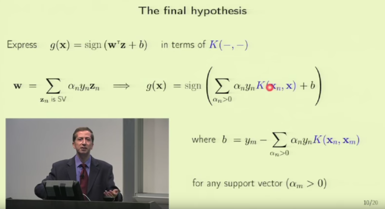
And to finally obtain and , we need to utilize kernel function too:
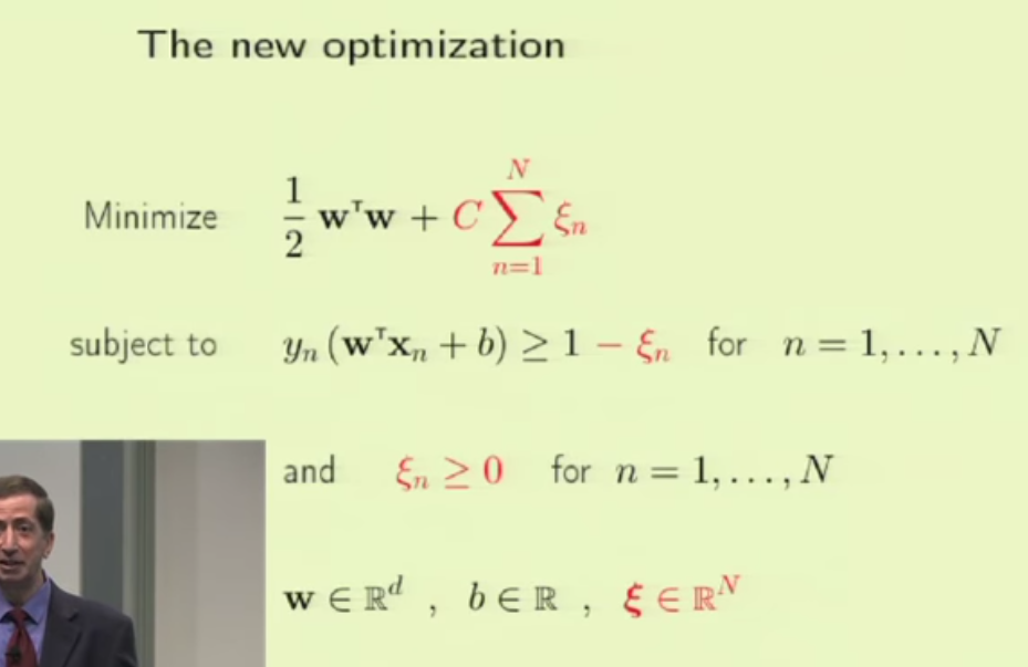
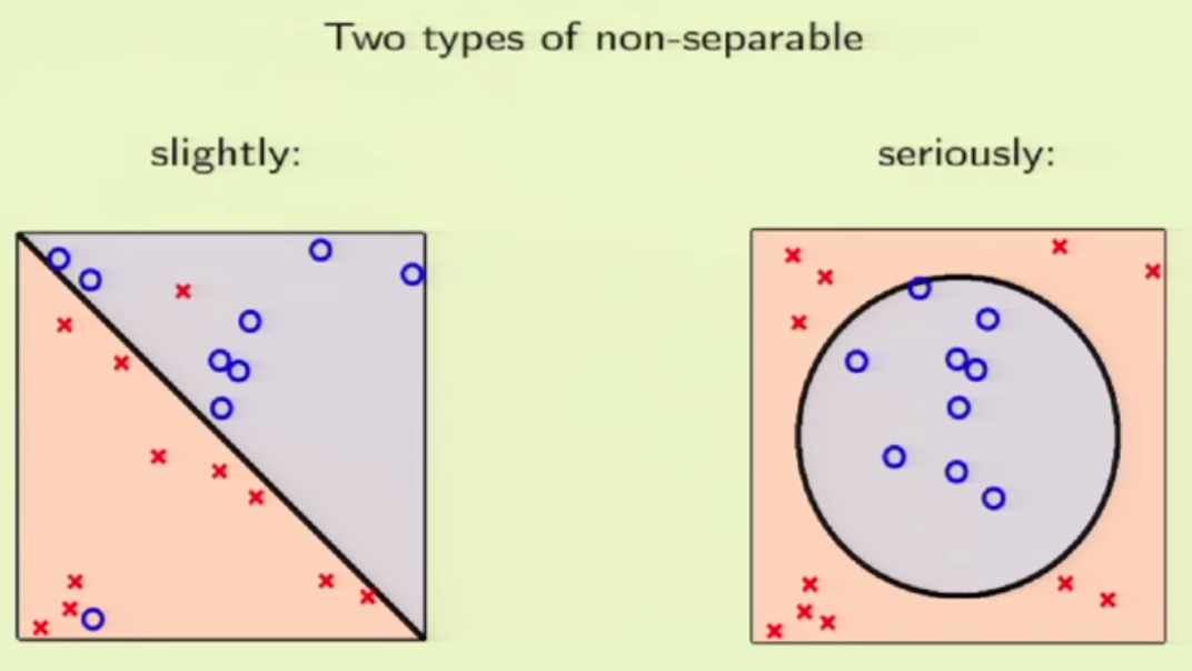
The second solution to deal with non-linearly separable problems is to use soft-margin. The intuition is to allow some violation of the margin constraint for some data points.
To compare the two solutions, we find that the kernel solution is often used when data are highly non-linearly separable. The soft-margin SVM is often used when data is just slightly non-linearly separable (most data are still linearly separable).
About practical issues of applying SVM, please refer to [3].
Reference
[1] lectures from Caltech online ML course
https://www.youtube.com/watch?v=eHsErlPJWUU
and
https://www.youtube.com/watch?v=XUj5JbQihlU
[2] https://czxttkl.com/?p=1449
[3] https://www.csie.ntu.edu.tw/~cjlin/papers/guide/guide.pdf
[4] http://www.cmap.polytechnique.fr/~mallat/papiers/svmtutorial.pdf
[5] https://stats.stackexchange.com/questions/239912/lagrange-multipler-kkt-condition
[6] https://www.cs.cmu.edu/~epxing/Class/10701-08s/recitation/svm.pdf
[7] convex optimization textbook: https://www.dropbox.com/s/fk992yb6qja3xhv/convex%20optimization.pdf?dl=0
Some chinese references:
[a] http://www.cnblogs.com/jerrylead/archive/2011/03/13/1982639.html