It is a cool idea that we can formulate data of many problems as graphs. It is even cooler that we can improve graph-based algorithms with Reinforcement Learning (RL). In this post, I am going to overview several related ideas.
Warm up on graphs – GCN
Let’s first warm up with some contexts on graphs. Graphs are everywhere; many data can be represented in a graph format. Graphs provide richer information than simple feature engineering because each node’s neighborhood information may be very valuable for characterizing a node thus being very valuable for prediction tasks. One famous graph model is called Graph Convolutional Networks (GCN) [3] ([4, 5, 6] are good tutorials).
In GCN, nodes are represented as vectors, which we denote as  , with
  being the number of total nodes and
  is the vector dimension. We hope to learn these vector representations using
  layers of neural networks. A simple learning rule (in [3] it is called propagation rule) is:
 ,
,
where  is the adjacency matrix,
  is the node representation from the previous layer,
  is an activation function, and
  is the parameters of this layer.
  is some basic feature representation of nodes, which can be as simple as an identity matrix, or as complex as shortest path distance to other nodes.
The problem of the simple propagation rule is that: (1) the computation of  does not involve each node’s own representation; (2) nodes with large degrees will tend to have large values in their feature representation while nodes with small degrees will have small values. Therefore, a better propagation rule is:
 ,
,
where  ,
,  is the inverse degree matrix of
  as a way to normalize the following value by the degree of each node.
In [3], the authors further proposes  , which has some theoretical connection to “localized spectral filters”. This form of propagation rule, according to [5], not only takes into considerations the degree of the source node but also the target node for each node pair.
It is important to note that node representation  can be learned by unsupervised learning or semi-supervised learning manner. What we describe above is the unsupervised learning approach, in which node embeddings are computed without knowing any node labels. A more interesting point of [3] is that the propagation rule can be used to learn node representation in a semi-supervised learning setting, where only some nodes’ labels are revealed but the representations of all the nodes in the graphs can be learned. This is because if we back-propagate on the prediction loss function, it can eventually back-propagate to all other nodes due to that the nodes with labels have representations as the aggregation from other nodes’.
Knowledge Graphs
Knowledge graphs can be seen as a special form of graphs: graphs with heterogenous types of edges. Using knowledge graphs can help on many downstream tasks. I happen to know two works which use knowledge graph information to aid recommendation system tasks.
The first work is called Deep Knowledge-Aware Network (DKN) [7]. It solves the problem of news recommendation. If we don’t use knowledge graphs, for each news candidate and for each historical read news article from a specific user, we can only featurize it by text information. The authors propose to map entities mentioned in news titles to a pre-built knowledge graph and create the entity representation in the knowledge graph. Then they can augment each news article’s feature representation with the entity representation from the entities mentioned in the news title. With the augmented feature representation, retrieval/ranking tasks can be more accurate.
While [7] can be thought of as a content-based method to aid recommendation, [8] is a structure-based method, i.e., it uses structure information of nodes in a graph neural network to help predicting CTR/engagement. Node embeddings are learned from a GCN-based approach on a pre-built knowledge graph, as GCN is a suitable algorithm for distilling neighborhood structures. (Note [7] and [8] are from the same group of authors who rely on Microsoft Satori knowledge graph system). Also, to avoid huge memory consumption, they don’t use the adjacency matrix in the computation, but instead sampling a fixed number of neighborhoods when aggregating each node’s representation from its neighbor.
There are many ways to learn node embeddings in knowledge graphs. Top famous ones are (the screenshot is from [7], which gives a good overview):
Markov Chains on graphs
Now, let’s look at some problems where Markov Chains are formulated on graphs. In a paper from Spotify [1], the authors assume that users’ interactions with different music genres are a Markov chain:

where  is the distribution of user
  ‘s played genres at time
  . Hence, can be represented as play counts on each genre
 ![\mathbf{n}^t_i=[n^t_{i1}, \cdots, n^t_{iN}]](https://czxttkl.com/wp-content/ql-cache/quicklatex.com-15ceafaa5104efb08d21a81fb48771d2_l3.png "Rendered by QuickLaTeX.com") normalized by total play counts
normalized by total play counts  :
:  . The transitions between genres at different time steps are considered as a graph.
Then, they use some traditional graph models to formulate the generative process of and  :
:


The core idea is that:
1. The total play count at time step  ,
,  , is sampled from a Poisson distribution determined by .
2. The play count on each category on the next timestep,  , will then be determined by both the total play count and the genre distribution
  . is a
  transition matrix to be learned denoting how user genre preferences change in two consecutive steps. The paper chooses to use some two-step maximal likelihood method to learn and
  .
.
A much older paper [2] bears the same idea, where it learns item-to-item transitions instead of genre transitions.
Random Walk
Random walk is a powerful algorithm. With proper parameterization, random walk is essentially the same as personalized page-rank [16]. Many graph learning techniques also rely on random walk as an important component.
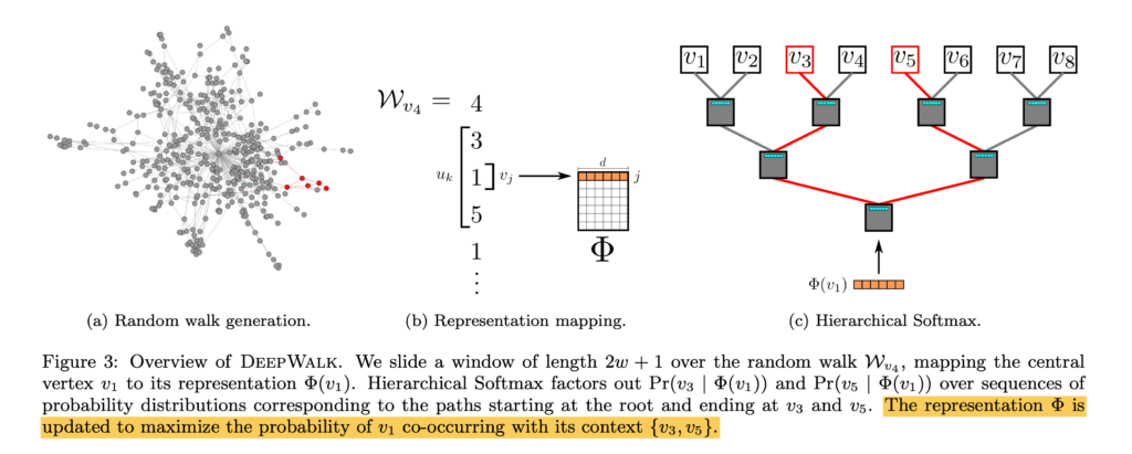
DeepWalk [9] uses node visit sequences from random walk to learn node representation. Its idea can be illustrated in the diagram below. Suppose from node 3, a random walker can reach to 1, 5, 1, …. We can use a fixed-size moving window to examine each node: for example, when we are at node 1 whose neighbors in the random walk sequence is node 3 and 5, we wish to predict the context node 3 and 5 given the representation of node 1. The model structure will be similar to SkipGrams which is widely used in NLP. The paper has some computation optimization on the prediction layer (softmax layer), which turns normal softmax into hierarchical softmax.
Node2Vec [11] is another similar work to DeepWalk. The only difference is that DeepWalk uses the pure random walk to generate node visitation sequence, whereas Node2Vec has two hyper-parameters to control the random walk tendency to favor breadth-first search v.s. depth first search [10].
Markov Decision Process on Graphs
Applying RL on graphs means we need to formulate a Markov Decision Process. The common idea is to learn to navigate in the graph such as to reach a desired node. Here is a knowledge graph-based application from MINERVA [13].
The idea of MINERVA is that if we want to query a knowledge graph by (source node, relationship), we want to land on a target node which could give us the answer. For example, source node=Obama, relationship=nationality, we want to learn an agent to traverse the graph and eventually land on the node=United States. The sequence of node navigation can be seen as a sequential decision problem: the agent, based on its current state and available outgoing relationships, needs to decide which next node to go to. So this agent can be naturally learned by reinforcement learning. Since the knowledge graph query task usually has ground truth data {(source node relationship, target node)} , we can design the reward function to be +1 if the agent eventually lands on the target node, or -1 if not.
DeepPath [12] is similar to MINERVA but simpler. DeepPath learns to return an efficient reasoning path that connects the source and target node (hence its each state always contains source and target node and the query relationship), whereas MINERVA always only contains source node and the query relationship. There is also a similar work [14] which improves the sample efficiency of RL-based walkers.
References
[1] Where To Next? A Dynamic Model of User Preferences: https://dl.acm.org/doi/10.1145/3442381.3450028
[2] Factorizing Personalized Markov Chains for Next-Basket Recommendation: https://dl.acm.org/doi/abs/10.1145/1772690.1772773
[3] Semi-Supervised Classification with Graph Convolutional Networks: https://arxiv.org/abs/1609.02907
[4] https://towardsdatascience.com/how-to-do-deep-learning-on-graphs-with-graph-convolutional-networks-7d2250723780
[5] https://towardsdatascience.com/how-to-do-deep-learning-on-graphs-with-graph-convolutional-networks-62acf5b143d0
[6] https://csustan.csustan.edu/~tom/Clustering/GraphLaplacian-tutorial.pdf
[7] DKN: Deep Knowledge-Aware Network for News Recommendation: https://arxiv.org/abs/1801.08284
[8] Knowledge Graph Convolutional Networks for Recommender Systems: https://arxiv.org/abs/1904.12575
[9] DeepWalk: Online Learning of Social Representations: https://arxiv.org/abs/1403.6652
[10] https://antonsruberts.github.io/graph/deepwalk/
[11] Node2Vec: https://arxiv.org/abs/1607.00653
[12] DeepPath: A Reinforcement Learning Method for Knowledge Graph Reasoning: https://arxiv.org/abs/1707.06690
[13] Go for a Walk and Arrive at the Answer: Reasoning Over Paths in Knowledge Bases using Reinforcement Learning: https://arxiv.org/abs/1711.05851
[15] M-Walk: Learning to Walk over Graphs using Monte Carlo Tree Search: https://arxiv.org/abs/1802.04394
[16] https://www.r-bloggers.com/2014/04/from-random-walks-to-personalized-pagerank/
 , where
  .
.


 is the change (i.e., derivative) of the hidden state.
 and
and  when we assume the input function
  becomes the sequence
  , where
  is the step size.


 . You would like to express the distribution of
  . You have some prior
  . You would like to know the distribution of the posterior distribution
  . Based on Bayes’ theorem,
![\[p(\theta|x)=\frac{p(\theta) p(x|\theta)}{p(x)}=\frac{p(\theta) p(x|\theta)}{\int_\theta p(\theta) p(x|\theta) d\theta}\]](https://czxttkl.com/wp-content/ql-cache/quicklatex.com-2529e21a8f21d8b383b095d0962a740d_l3.png "Rendered by QuickLaTeX.com")
 is often hard to compute. Therefore, it is hard to know the exact statistics of the posterior distribution, such as the mean of the posterior distribution. MCMC has some mechanism to allow you sample points on the space of
  while
while  is a fixed variance. According to basic conjugate prior mathematics [4], you have a prior distribution
  which is also a Normal distribution. You have observed 3 students’ scores therefore you can express the likelihood function as:
  . In this simple example, there is an analytical expression for the posterior distribution
  which is also a Normal distribution. But for our pedagogical purpose, let’s assume the posterior distribution
  is impossible to compute and we have to use MCMC to infer posterior statistics such as the posterior mean.
  at first.
 is defined in [1].
 and
and  .
. ![\[\alpha(\theta^{new}, \theta^{old})=min \left(1, \frac{p(\theta^{old}|x)g(\theta^{new}|\theta^{old})}{p(\theta^{new}|x) g(\theta^{old}|\theta^{new})}\right)\]](https://czxttkl.com/wp-content/ql-cache/quicklatex.com-75a1b765204a57aa4e742b7c38f731ef_l3.png "Rendered by QuickLaTeX.com")
 for
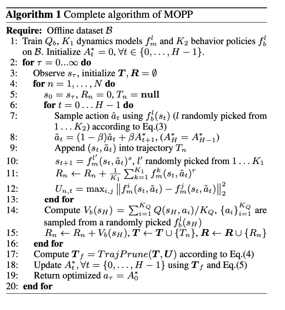
for  . Each behavior cloning model models the output action as a normal distribution with a predicted mean and standard deviation. Each time when we want to sample an action, we first randomly pick a behavior cloning model and then sample the action multiple times according to the predicted mean and standard deviation. However, there is some additional adaptation for how to sample from the predicted mean and standard deviation. First, the standard deviation is scaled larger so that action sampling can be more diverse and aggressive. Second, to counter sampling bad actions, we learn a Q-function from logging data and use it to finally select the action to proceed the trajectory simulation. Although the Q-function estimates the Q-value for the behavior policy instead of the policy being learned, the authors argue that it “provides a conservative but relatively reliable long-term prior information”. The two points are manifested in Eqn. 3:
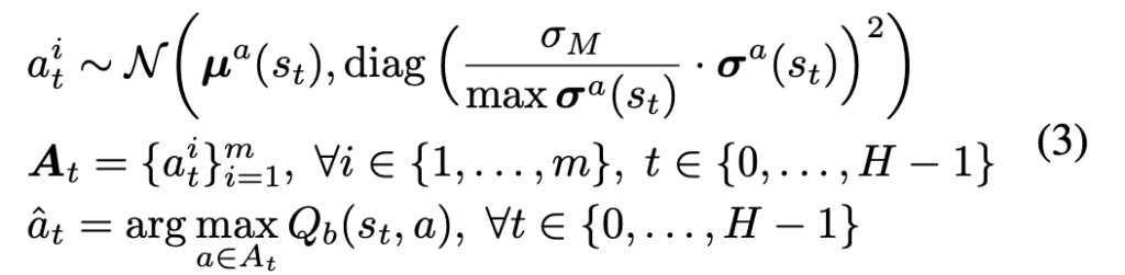
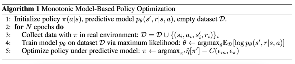
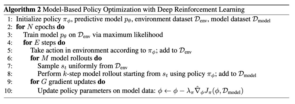
 , the largest disagreement between any two dynamic models in the ensemble.
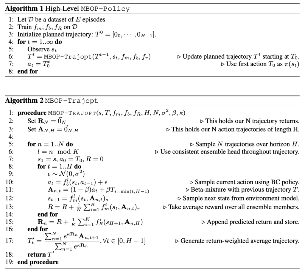
 Note one detail at line 14: if we simulate
  steps, we can get
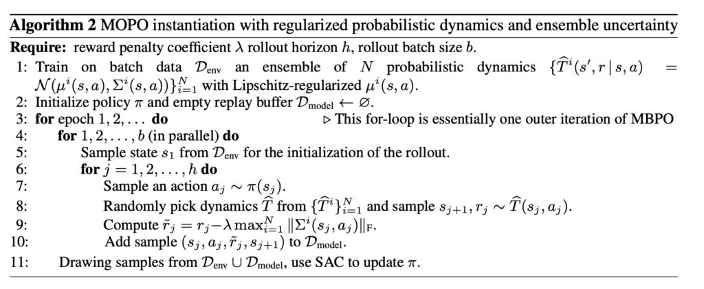
 , the maximum standard deviation of the learned models in the ensemble. As the authors argue, “empirically the learned variance often captures both aleatoric and epistemic uncertainty, even for learning deterministic functions (where only epistemic uncertainty exists). We use the maximum of the learned variance in the ensemble to be more conservative and robust.”
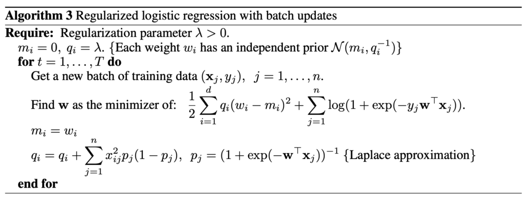
 . We have a dataset
  which contains tuples of
  for
for  . These are observed features and labels. If we apply a Bayesian logistic regression on such data, the logistic regression will have a weight vector of the same dimension as the features:
  . The prediction function is a sigmoid function:
  .
. given the observation
  . We assume that
  .
. 

 , what would be
  and
and  ?
?
 achieves maximum
  , which is able to be found using gradient ascent or expressed in a closed formula (I think
  . Because
  , we can further simplify to
  .
.  can actually be seen as the logarithm of another Gaussian distribution
  , whose mean is at
  , and
, and  absorbs any remaining constants. This is why Algorithm 3 updates
  because
  is essentially from
  since this is essentially
  .
.