Laplacian Approximation and Bayesian Logistic Regression

Recently, I am studying a basic contextual bandit algorithm called Logistic Regression Bandit, which is also known as Bayesian Logistic Regression. It all starts from the paper “An Empirical Evaluation of Thompson Sampling” [1]. In Algorithm 3 in the paper, the authors gives the pseudo-code for how to train the Logistic Regression Bandit, assuming its weights are from a Gaussian distribution with a diagonal covariance matrix:

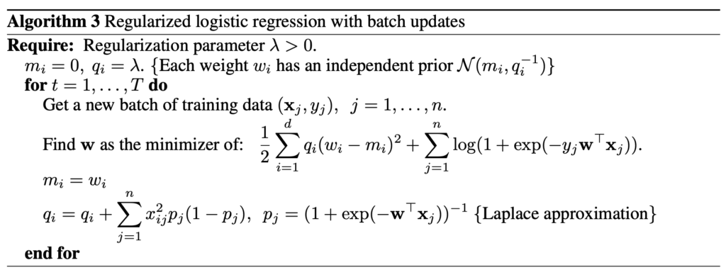
When I first read it, my biggest confusion is Laplace approximation – why is it used in training a Bayesian logistic regression? Now, let’s dig into how Laplace approximation comes into play.

Let’s first review the set up of a Bayesian logistic regression. Suppose we have a feature space $\mathbf{x} \in \mathbb{R}^d$ . We have a dataset $\mathcal{D}$ which contains tuples of $(\mathbf{x}_i, y_i)$ for $i=1, \cdots, N$ . These are observed features and labels. If we apply a Bayesian logistic regression on such data, the logistic regression will have a weight vector of the same dimension as the features: $\mathbf{w} \in \mathbb{R}^d$ . The prediction function is a sigmoid function: $p(\mathbf{x}) = \left( 1+exp(-\mathbf{w}^T\mathbf{x})\right)^{-1}$ .

Because it is a Bayesian logistic regression, we need to estimate a posterior probability distribution for $\mathbf{w}$ given the observation $\mathcal{D}$ , $p(\mathbf{w}|\mathcal{D})$ . We assume that $\mathbf{w}$ come from a multi-dimensional Gaussian distribution with a diagonal covariance matrix. This is the same as what Algorithm 3’s notation implies: $w_i \sim \mathcal{N}(m_i, q_i^{-1})$ .

We can also get the likelihood function $p(\mathcal{D}|\mathbf{w})=\prod\limits_{j=1}^N p(\mathbf{x}_j)^{y_j} \left(1-p(\mathbf{x}_j)\right)^{1-y_j}$

Using the Bayesian Theorem, we can derive (the notations adapted from [2] (slides page 9~12) to the notations in this post):

$p(\mathbf{w}|\mathcal{D}) \propto p(\mathbf{w})p(\mathcal{D}|\mathbf{w})\newline\quad\qquad=\prod\limits_{i=1}^d \mathcal{N}(m_i, q_i^{-1}) \prod\limits_{j=1}^N p(\mathbf{x}_j)^{y_j} \left(1-p(\mathbf{x}_j)\right)^{1-y_j}$

Now, here is how Lapalace Approximation [3] comes into play. The goal of Lapalace Approximation is to learn a Gaussian distribution to approximate $p(\mathbf{w}|\mathcal{D})$ , which is not a Gaussian distribution in its exact expression. In other words, if $p(\mathbf{w}|\mathcal{D}) \approx \mathcal{N}(m_i', q_i'^{-1})$ , what would be $m_i'$ and $q_i'$ ?

First, we will take the logarithm on both sides, leading to:

$\log p(\mathbf{w}|\mathcal{D}) = -\left( \frac{1}{2}\sum\limits_{i=1}^d q_i (w_i - m_i)^2 + \sum\limits_{j=1}^n \log(1 + exp\left( -y_j \mathbf{w}^T \mathbf{x}_j\right)) \right) + const \newline= f(\mathbf{w}) + const$

Suppose $f(\mathbf{w})$ achieves maximum $\mathbf{w}_0$ , which is able to be found using gradient ascent or expressed in a closed formula (I think $f(\mathbf{w})$ is a concave function but not totally sure). Based on the 2nd-order Taylor expansion at point $\mathbf{w}_0$ , we have: $f(\mathbf{w}) \approx f(\mathbf{w}_0) + f'(\mathbf{w}_0)(\mathbf{w}-\mathbf{w}_0)+\frac{1}{2}f''(\mathbf{w}_0)(\mathbf{w} - \mathbf{w}_0)^2$ . Because $f'(\mathbf{w}_0)=0$ , we can further simplify to $f(\mathbf{w}) \approx f(\mathbf{w}_0) +\frac{1}{2}f''(\mathbf{w}_0)(\mathbf{w} - \mathbf{w}_0)^2$ .

$f(\mathbf{w}_0) +\frac{1}{2}f''(\mathbf{w}_0)(\mathbf{w} - \mathbf{w}_0)^2$ can actually be seen as the logarithm of another Gaussian distribution $\mathcal{N}(m_i', q_i'^{-1})$ , whose mean is at $\mathbf{w}_0$ and variance as $-f''(\mathbf{w}_0)$ , and $f(\mathbf{w}_0)$ absorbs any remaining constants. This is why Algorithm 3 updates $m_i = w_i$ because $w_i$ is essentially from $\mathbf{w}_0$ that maximizes $f(\mathbf{w})$ , and $q_i=q_i + \sum\limits_{j=1}^n x^2_{ij}p_j(1-p_j)$ since this is essentially $f''(\mathbf{w}_0)$ .