In this post, we review the concept of data parallelism, model parallelism, and more in between. We will illustrate ideas using SOTA ML system designs.
Data Parallelism
Data parallelism means that there are multiple training workers fed with different parts of the full data, while the model parameters are hosted in a central place. There are two mainstream approaches of doing data parallelism: parameter servers and AllReduce.
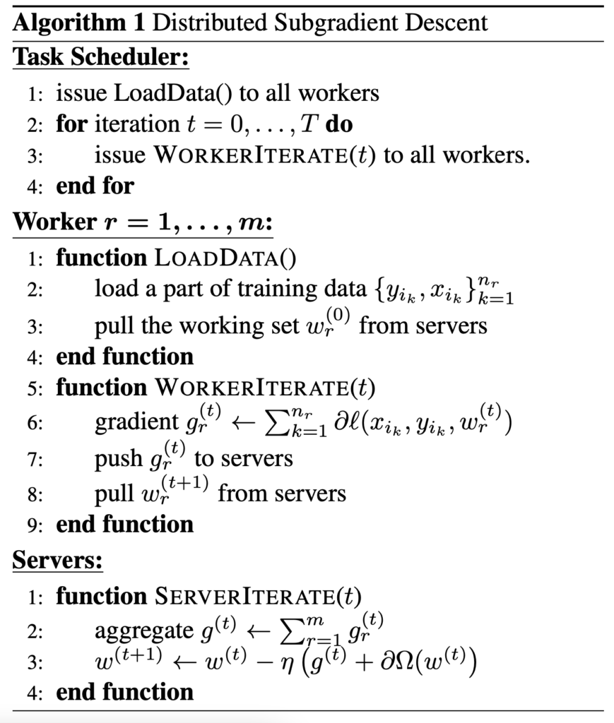
Parameter Servers host model parameters in a server node group. Its basic form is illustrated in the pseudocode below. We can see that workers do not hold any model parameter. They only push local gradients to servers and fetch weights from servers afterwards, while there is no communication between workers.
I covered Ring AllReduce in my previous post [1] (when I surveyed the Ray paper). In short, Ring AllReduce aggregates the gradients of the model parameters between all training nodes after every round of training (i.e., one minibatch on each trainer node). In PyTorch, it is implemented in an API called DistributedDataParallel [2]. Each training node will have a full copy of the model and receive a subset of data for training. Once each node has one forward pass and the corresponding backward pass, the model parameters’ gradients will be synced using the AllReduce primitive. Such behaviors are studied in my previous post [3].
[2] makes a distinction between AllReduce and Parameter Servers: As one AllReduce operation cannot start until all processes join, it is considered to be a synchronized communication, as opposed to the P2P communication used in parameter servers. Hence, from this distinction, you can see that the communication cost of parameter servers grow linearly with the number of trainer nodes in the system. On the other hand, Ring AllReduce is an algorithm for which the communication cost is constant and independent of the number of trainer nodes in the system, and is determined solely by the slowest connection between trainer nodes in the system [15]. There is an empirical report comparing Ring AllReduce and Parameter Servers [14]. The result is consistent with our analysis: “it is easy to see that ring all-reduce (horovod) scales better on all models”.
Model Parallelism
The vanilla model parallelism is just to hold different parts of a model on different devices. It is useful when you have a model too large to be held on one node.
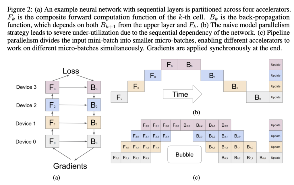
Pipeline parallelism [4] is a more advanced method of model parallelism which can have great speed-up over the vanilla model parallelism. First, the layers of a model are partitioned into a series of “cells”. Each cell is placed on a different node. Then, a mini-batch is split into smaller batches, called micro-batch, which get fed to cells in a sequential way such that each cell is operating on a micro-batch at one time. Therefore, the time for waiting for data to be processed on other nodes is minimized. The idea of pipeline parallelism is best illustrated in the diagram below (subplot c):
To put data parallelism and pipeline parallelism into a more concrete context, let’s study the paper PipeTransformer [5], which employs a hybrid of data parallelism and model parallelism. PipeTransformer employs synchronous pipeline parallel within one machine and data parallel across machines. It gradually freezes the stack of layers in order to reduce the number of active parameters, and spawns more processes on freed resources to increase data parallel width. PipeTransformer combines four components: Freeze Algorithm, AutoPipe, AutoDP, and AutoCache.
- Freeze Algorithm, which is responsible for determining until which layer from the bottom should be frozen. Freezing layers comes from the recent study that parameters in neural networks usually converge from the bottom-up. After a few iterations, the bottom layers usually start to the less actively changed through the end of the training.
- AutoPipe, which will create cell partitions among the unfrozen layers. The size of a cell will be adjusted smartly for best speed. For example, pipelines can be compressed (i.e., cells can be merged) to reduce the bubble size, which is the speed bottleneck for a pipeline. Because of Freeze Algorithm and techniques in AutoPipe, as the training goes on and more layers are frozen, one pipeline will occupy less nodes (e.g., GPUs).
- AutoDP, which can create data parallelism either on the same machine or across machines. Data parallelism across machines is easy to understand because it naturally increases the throughput of training. On the other hand, data parallelism on the same machine is possible because AutoPipe will dynamically reduce the size of pipelines on one machine so there could be more replicas of pipelines even on the same machine.
- AutoCache is more specific to the freezing training paradigm because caching frozen layers’ outputs could skip the same computation over and over again.
I find the diagram below is useful for illustrating AutoPipe and AutoDP:


While this post cannot survey all relevant papers, I find the table from [2] is comprehensive (at least as of 2021):


Practical Examples
There are some more practical lessons I learned from Pytorch official document.
CUDA semantics [6]
Each cuda device maintains a default stream. Within the same stream, operations are executed sequentially. But across different streams, operations are executed asynchronously. So if you modify a tensor on cuda:0 and then modify another tensor on cuda:1, do not assume that you can see the change to the tensor on cuda:0 if you have seen the change to the tensor on cuda:1.
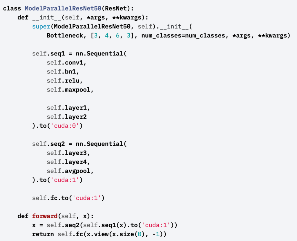
Single-Machine Model Parallelism [7]
On a single machine, the vanilla model parallelism is to place different parts of a model to different cuda devices. As an example:
To use the pipeline parallelism, one needs to further split mini-batches into micro-batches and feed different micro-batches into different parts of the model. As an example:
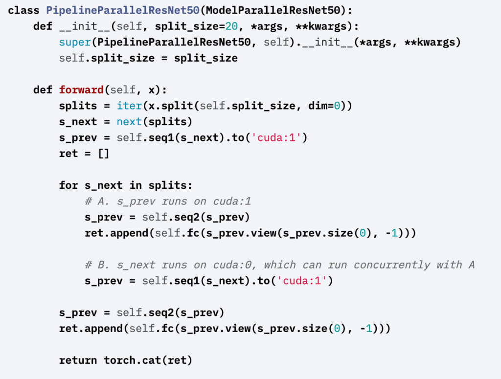
As we can see, the vanilla model parallelism introduces more communication overhead. When a model can just fit into one gpu, the vanilla model parallelism actually has a worse speed than not using it. Pipeline parallelism can speed up things but the speed up is only sub-linear because of extra overhead.

Later, I found that Pytorch has a wrapped class called Pipe to handle pipeline parallelism automatically. Here is an example of using Pipe to train a Transformer model [9].
Use rpc to implement parameter servers
I find there are three good examples for how rpc can be flexible to implement a parameter server.
In the first example [10], they create a parameter server in one process. The parameter server holds a nn.Module. This module has different partitions on different gpu devices. There are two trainer processes. In each of them, a TrainerNet is created for passing input to the module on the parameter server process through rpc remote call. As you can see, the forward function of TrainerNet is purely a rpc remote call. In other words, there is no linear algebra computation happening on the trainer processes in this example. The overall training loop (run on each trainer process) is very simple. A DistributedOptimizer is used to optimize model parameters (hosted remotely on the parameter server process).
In the second example [11], they implement a training script that support both a parameter server and data parallelism. There are four processes: one master process, one parameter server process, and two trainer processes. It is best to read the training script from the master process. The master process first creates a RemoteModule on the parameter server process. Then it uses the rpc_async API to start _run_trainer method on two trainer processes. The master process passes the reference to the RemoteModule to _run_trainer. Therefore, each trainer process can use the reference to create a HybridModel, which holds both the reference to the RemoteModule and some local model synced by DistributedDataParallel. Things become clear if you look at the forward function of HybridModel: data are passed to the RemoteModule first and then to the local model to generate model outputs.
The third example [12] is simpler than the previous two. There is one parameter server process and one trainer process. It is easier to understand the script by starting from the trainer process. The trainer process first initializes an RNN model, which holds some local LSTM module and the remote reference to an EmbeddingTable and a Decoder. The EmbeddingTable and Decoder are created on the parameter server process through rpc remote call.
Use rpc to implement agent-observer reinforcement learning paradigm
This pedagogical example [13] is interesting because it shows how rpc remote calls happen between several processes back and forth. First of all, there is an agent process and several observer processes. The agent holds the remote reference to Observer class, which is created on every observer process. When the agent needs to collect rl training data, it kicks off run_episode method of Observer on the observer processes. While in the run_episode method of Observer, we call the agent’s select_action and report_reward methods through rpc remote calls. Hence you can see that there are multiple rpc remote calls between the agent process and observer processes.
——————————- Update 2022-01-03 ——————————-
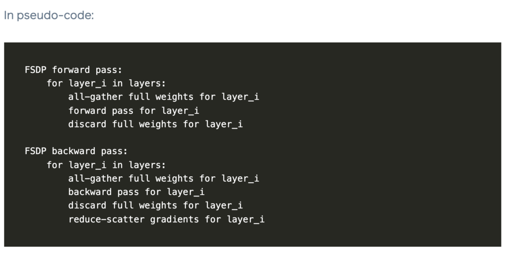
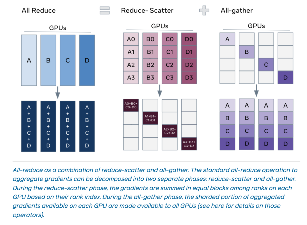
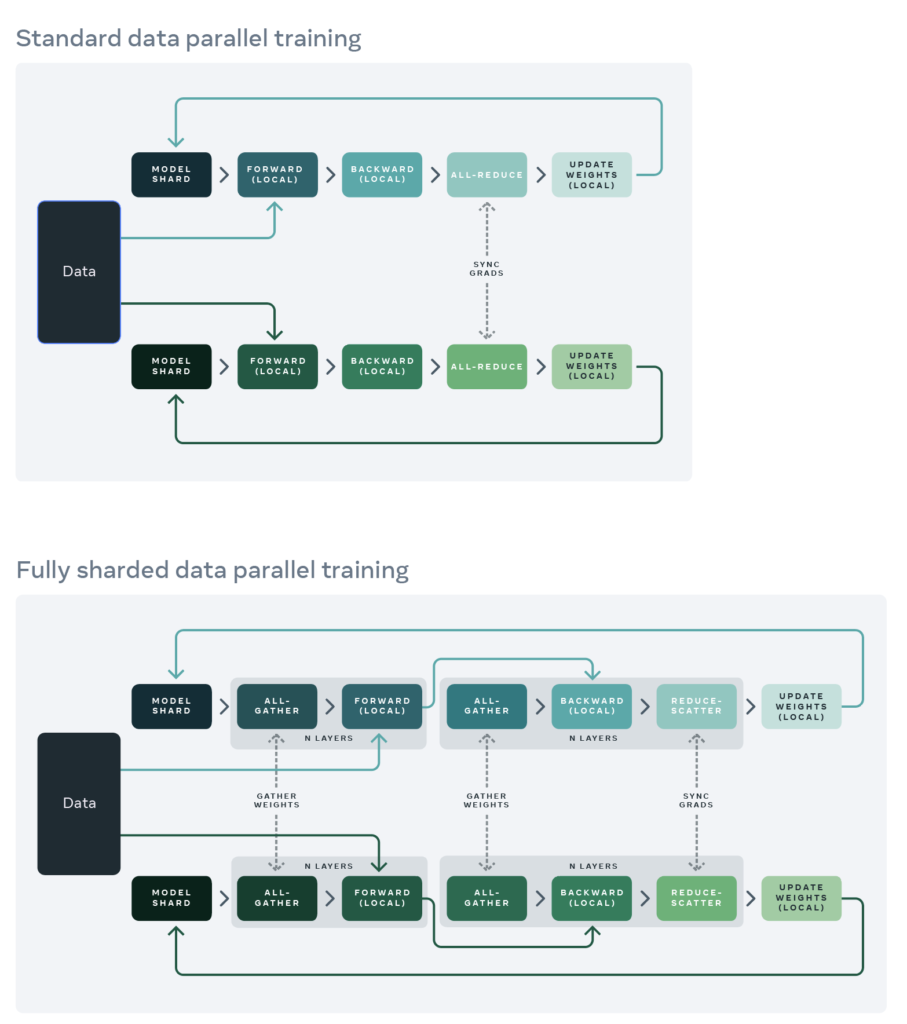
I want to take down some notes about the ZERO paper [16] because it introduces some basic concepts about data and model parallelism. We start from recalling DistributedDataParallel which implements All-Reduce (see Data Parallel and DistributedDataParallel in “Data Parallelism” section; see introduction of All-Reduce in [1]). Typically, each process in an All-Reduce group will hold memory as much as all the parameters and other optimizer states would take, even though at each round of All-Reduce each process is only responsible for storing one shard of all the parameters correctly.
Therefore, the basic idea of ZERO (which is also called Fully Sharded Data Parallel (FSDP) at Meta [17]) is to only keep one shard of parameters in the memory; when forward and backward computation need to know the values of other shards, the all-gather operator is used to construct necessary parameters on the fly. I think the pseudo-code from [17] best describes the ZERO or FSDP:
The ZERO paper has some good explanation on memory usage during the lifecycle of model training. Based on Section 3 (Where did all the memory go?), I summarize three main memory usages: (1) parameters & gradients; (2) optimizer states, such as momentum/variance as required by Adam; (3) residual states, such as activations.
If we apply FSDP on parameters, gradients, and optimizer states in a setting of mixed-precision training with Adam optimizer, then ZERO would have ~60x reduction in memory if we use  GPUs, as shown in the table below, where
  ,
,  , and
, and  means we apply ZERO only on optimizer states, gradients, and parameters, respectively:

For activations, we need to first illustrate why activations occupy memory in model training. This is because during backprogagtion, we need to both activation values and model parameter values to compute derivatives. If we do not store activations computed in the forward pass, we then need to recompute them in the backward pass. Therefore, a straightforward method is to save all activations computed in the forward pass for later usage in the backward pass. As you can see, this would require GPU memory as much as all activations. Only when backpropagation has progressed long enough to have all dependencies of an activation computed can the activation be discarded.
It is a usual practice to apply activation checkpoints, a technique to reduce memory footprints of activations (see [18] for a good tutorial). Activation checkpointing store only a subset of activations, allowing activations to be recomputed but not too often. The most memory-efficient way to checkpoint activations is to store every sqrt(n) activations, where n is the number of total layers. ZERO applies FSDP on activations to have them sharded on different GPUs.
As you may see from the pseudocode and explanations above, ZERO/FSDP can reduce the memory optimizer states and activations by sharding to different GPUs, which is not done in DistributedDataParallel. However, the peak memory will still depend on the parameters/activations after all-gather at some points in forward/backward. Note that, all-gather usually only gather parameters/activations per layer. So ZERO/FSDP will enjoy the most memory reduction if you can break down your models into many layers.
In 04/2021, Microsoft released a new blog post about ZERO-infinity, which is based on ZERO plus several enhancement: https://www.microsoft.com/en-us/research/blog/zero-infinity-and-deepspeed-unlocking-unprecedented-model-scale-for-deep-learning-training/
——————————- Update 2022-01-03 ——————————-
todo: https://thegradient.pub/systems-for-machine-learning/
References
[1] https://czxttkl.com/2020/05/20/notes-on-ray-pap/
[2] PyTorch Distributed: Experiences on Accelerating Data Parallel Training
[3] Analyze DistributedDataParallel (DPP)’s behavior: https://czxttkl.com/2020/10/03/analyze-distributeddataparallels-behavior/
[4] GPipe: Efficient Training of Giant Neural Networks using Pipeline Parallelism
[5] PipeTransformer: Automated Elastic Pipelining for Distributed Training of Transformers
[6] CUDA semantics: https://pytorch.org/docs/stable/notes/cuda.html
[7] Single Machine Model Parallelism: https://pytorch.org/tutorials/intermediate/model_parallel_tutorial.html#speed-up-by-pipelining-inputs
[8] Pytorch RPC Framework: https://pytorch.org/docs/stable/rpc.html
[9] Train Transformers using Pipeline: https://pytorch.org/tutorials/intermediate/pipeline_tutorial.html
[10] IMPLEMENTING A PARAMETER SERVER USING DISTRIBUTED RPC FRAMEWORK: https://pytorch.org/tutorials/intermediate/rpc_param_server_tutorial.html, code: https://github.com/pytorch/examples/blob/master/distributed/rpc/parameter_server/rpc_parameter_server.py
[11] COMBINING DISTRIBUTED DATAPARALLEL WITH DISTRIBUTED RPC FRAMEWORK: https://pytorch.org/tutorials/advanced/rpc_ddp_tutorial.html, code: https://github.com/pytorch/examples/blob/master/distributed/rpc/ddp_rpc/main.py
[12] Distributed RNN using Distributed Autograd and Distributed Optimizer: https://pytorch.org/tutorials/intermediate/rpc_tutorial.html#distributed-rnn-using-distributed-autograd-and-distributed-optimizer, code: https://github.com/pytorch/examples/tree/master/distributed/rpc/rnn
[13] Distributed Reinforcement Learning using RPC and RRef: https://pytorch.org/tutorials/intermediate/rpc_tutorial.html#distributed-reinforcement-learning-using-rpc-and-rref, code: https://github.com/pytorch/examples/tree/cedca7729fef11c91e28099a0e45d7e98d03b66d/distributed/rpc/rl
[14] Analysis and Comparison of Distributed Training Techniques for Deep Neural Networks in a Dynamic Environment: https://www.diva-portal.org/smash/get/diva2:1224181/FULLTEXT01.pdf
[15] https://xzhu0027.gitbook.io/blog/ml-system/sys-ml-index/parameter-servers
[16] ZeRO: Memory Optimizations Toward Training Trillion Parameter Models: https://arxiv.org/pdf/1910.02054.pdf
[17] Fully Sharded Data Parallel: faster AI training with fewer GPUs: https://engineering.fb.com/2021/07/15/open-source/fsdp/