Some update before we dive into today’s topic: I have not updated this blog for about 2 months, which is considered a long time : ). This is because I have picked up more tech lead work for setting up the team’s planning. I sincerely hope that our team will steer towards a good direction from 2022 and beyond.
Now, let’s go to today’s topic: normalizing flows. Normalizing flows is a type of generative models. Generative models can be best summarized using the following objective function:
![\text{maximize}_{\theta} \quad \mathbb{E}_{x \sim P_{data}}\left[ P_{\theta}(x)\right],](https://czxttkl.com/wp-content/ql-cache/quicklatex.com-5fe9fcb62c0fc5ed93731b6ec6608093_l3.png "Rendered by QuickLaTeX.com")
i.e., we want to find a model  which has the highest likelihood for the data generated from the data distribution as such to “approximate” the data distribution.
According to [1] (starting 11:00 min), we can categorize generative models as:
- Explicit with tractable density. i.e.,
 has an analytical form. Examples include Normalizing Flows, PixelCNN, PixelRNN, and WaveNet. The latter three examples are autoregressive models which generate elements (e.g., pixels, audio clips) sequentially however are computationally heavy due to the nature of autoregressive. Normalizing Flows can generate the whole image instantaneously thus has a computational advantage over others. (For more pros/cons of Normalizing Flows, please refer to [4])
 - Explicit with approximate density, i.e., we are only optimizing for some bounds of . One example is Variational Encoder Decoder [2], in which we optimize ELBO.
- Implicit with no modeling of density. One example is Generative Adversarial Network (GAN), where we generate images just based on the generator network with a noise input.
Normalizing Flows is based on a theory called “change of variables” [3]. Suppose  and
and  are random variables both with dimension
  . Also, suppose there is a mapping function
  such that
  and
and  . Then the density functions of and have the following relationship:
 ,
,
where the last two equations are due to  . From now on, we assume that denotes data while denotes a random variable in a latent space.
In Normalizing Flows, the mapping is parameterized by (i.e.,  and
and  ), which is what we try to learn. The objective function for learning becomes:

As you can see, our goal is to learn to map complex data distribution into a simpler latent variable distribution (usually  ). The reason that we want to follow a simple distribution is that: first, we need to compute
  in the objective function so ideally
  should be easy to compute; second, once we learn , we know the mapping
  and
and  , and then we can easily sample
  and apply
  to generate new data (e.g., new images). The requirement for a valid and practical is that: (1) it has an invertible ; (2)
  or
or  is efficient to compute.
One nice property of Normalizing Flows is that you can chain multiple transformation  to form a new transformation. Suppose
  with each
  having a tractable inverse and a tractable Jacobian determinant. Then:
 , where
  .
.
In practice, we usually pick  and optimize for log likelihood. Therefore, our objective becomes (as can be seen in Eqn. 1 from the Flow++ paper (one SOTA flow model) [5]):

[6] provides a good tutorial for getting started in Normalizing Flows, while [7] has a more in-depth explanation and it will help a lot in understanding more advanced implementation such as Flow++ [8]. For now, I am going to introduce [6].
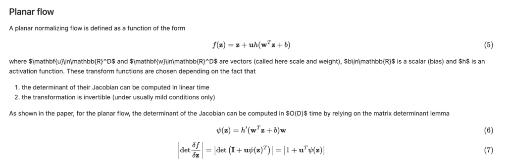
[6] introduces a flow called Planar Flow. It has relatively a straightforward transformation (linear + activation) and easy-to-compute Jacobian determinant:
Planar Flow is defined in Python as below:
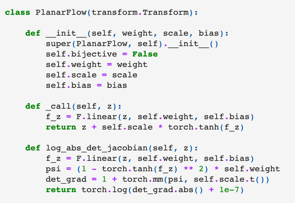
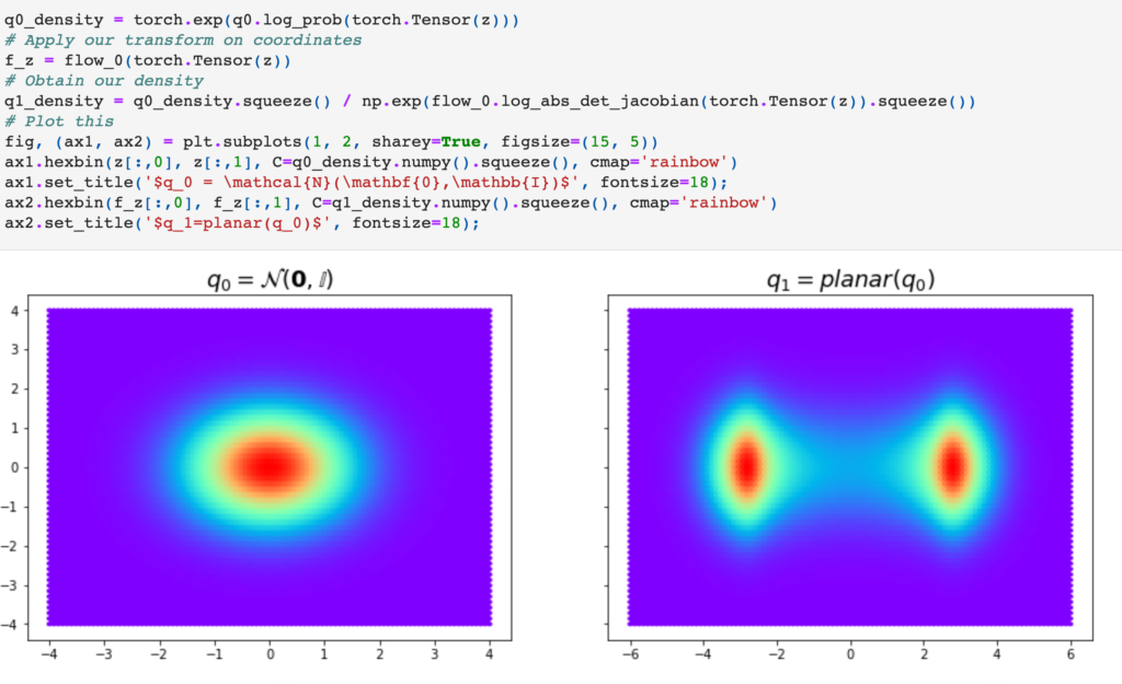
Once it is defined, we can instantiate an arbitrary Planar Flow and see how it transforms from a 2D Normal distribution:
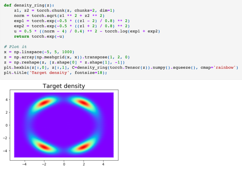
Now, suppose we want to learn what is the Planar Flow that could transform a 2D normal distribution to a target distribution defined as:
 The objective function, as we already introduced above, is
  . Here,
  is samples from a 2D normal distribution,
  is the target
 density_ring distribution. Therefore, the loss function (to be minimized) is defined as:

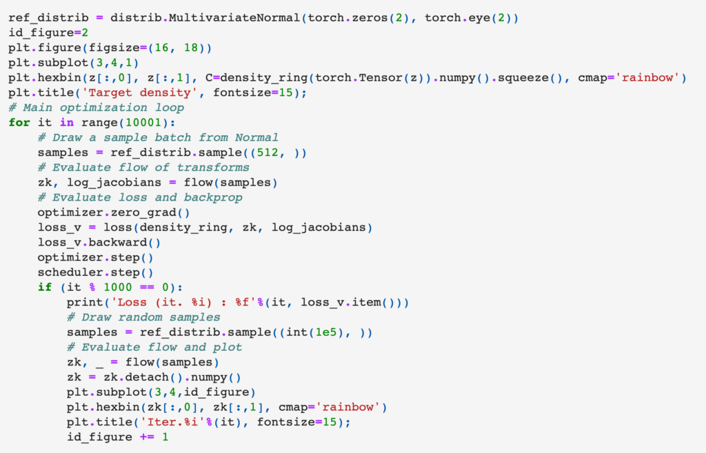
The overall training loop is:
Last, I highly recommend watching this ECCV tutorial: https://www.youtube.com/watch?v=u3vVyFVU_lI
TODO:
dequantization:
https://uvadlc-notebooks.readthedocs.io/en/latest/tutorial_notebooks/tutorial11/NF_image_modeling.html#Dequantization
https://arxiv.org/pdf/1511.01844.pdf
References
[1] PixelCNN, Wavenet & Variational Autoencoders – Santiago Pascual – UPC 2017 https://www.youtube.com/watch?v=FeJT8ejgsL0
[2] Optimization with discrete random variables: https://czxttkl.com/2020/04/06/optimization-with-discrete-random-variables/
[3] Normalizing Flows note: https://deepgenerativemodels.github.io/notes/flow/
[4] Introduction to Normalizing Flows: https://towardsdatascience.com/introduction-to-normalizing-flows-d002af262a4b
[5] Flow++: Improving Flow-Based Generative Models with Variational Dequantization and Architecture Design: https://arxiv.org/abs/1902.00275
[6] Normalizing Flows in PyTorch: https://github.com/acids-ircam/pytorch_flows/blob/master/flows_01.ipynb
[7] UvA DL Notebook: https://uvadlc-notebooks.readthedocs.io/en/latest/tutorial_notebooks/tutorial11/NF_image_modeling.html
[8] Flow++ Github implementation: https://github.com/chrischute/flowplusplus