Here, I am taking some notes down while following the GAN online course (https://www.deeplearning.ai/generative-adversarial-networks-specialization/).
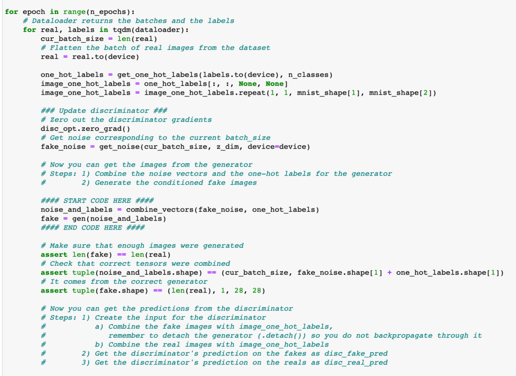
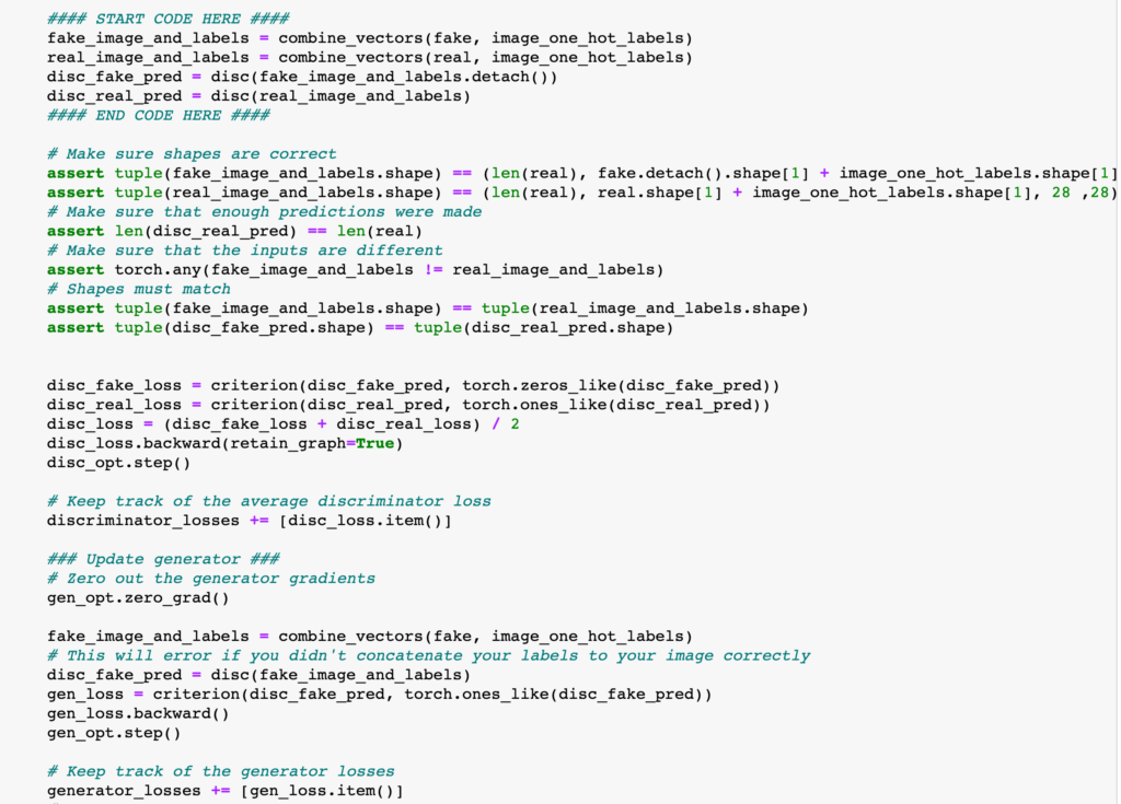
The first thing I want to point out is that one should be very careful about the computation graph during the training of GANs. To maximize efficiency in one iteration, we can call the generator only once, using the generator output to train both the discriminator and the generator itself. During training the discriminator, we need to call generator_output.detach(), so that after the discriminator loss is backward-ed, the gradient information of the generator is still kept in the computation graph for training the generator. Another option is to call `discriminator_loss.backward(retain_graph=True)` to keep the gradient information. You can see both methods in https://github.com/pytorch/examples/blob/a60bd4e261afc091004ea3cf582d0ad3b2e01259/dcgan/main.py#L230 and https://zhuanlan.zhihu.com/p/43843694.
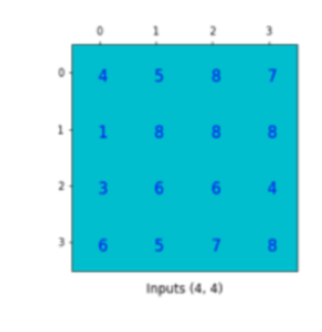
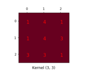
Next, we move to DCGAN (Deep Convolutional GAN) [1]. It is interesting to see that the generator/discriminator equipped with image-processing architectures like deconvolution/convolution layers will lead to more realistic generated images. The deconvolutional layer is something I am not familiar before. To understand it, we need to think of the convolution/deconvolution operation as matrix multiplication [2]. Suppose you have an input image (4×4) and a kernel (3×3), which expects to generate 2×2 output:
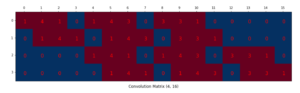
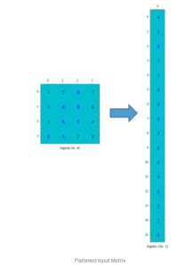
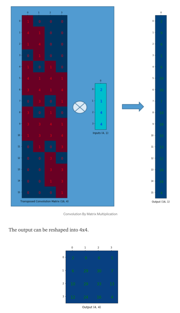
Equivalently, we can create a convolution matrix (4 x 16), flatten the input to (16 x 1), then multiply the two to get (4 x 1) output, and reshape to (2 x 2):
 .
. 

The deconvolution can be seen as the reverse of the convolution process. A 16×4 deconvolution matrix multiplies a flattened convoluted output (2 x 2 -> 4 x 1), outputting a 16 x 1 matrix reshaped to be 4 x 4.
The next topic is Wasserstein GAN [3]. The motivation behind it is that the original GAN’s generator loss (![max_g -\left[\mathbb{E}\left(log d(x)\right) +\mathbb{E}\left(1 - log d(g(z)) \right) \right]](https://czxttkl.com/wp-content/ql-cache/quicklatex.com-f94cdb5cdeb58b0480074930087633e2_l3.png "Rendered by QuickLaTeX.com") ) would provide little useful gradient when the discriminator is perfect in separating real and generated outputs. (There is much theory to dig in, but [4] gives a very well explanation on how it is superior in preventing mode collapsing and vanishing gradient.) The Wasserstein-loss approximates a better distance function than BCEloss called Earth Mover’s Distance which provides useful gradient even when the real and generated output is already separable.
) would provide little useful gradient when the discriminator is perfect in separating real and generated outputs. (There is much theory to dig in, but [4] gives a very well explanation on how it is superior in preventing mode collapsing and vanishing gradient.) The Wasserstein-loss approximates a better distance function than BCEloss called Earth Mover’s Distance which provides useful gradient even when the real and generated output is already separable.

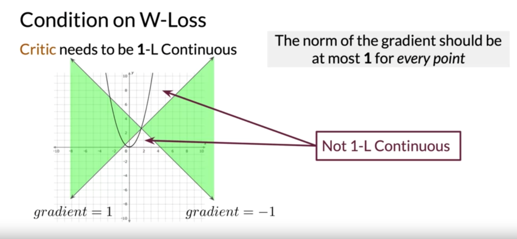
However, when training GANs using W-loss, the critic has a special condition. It has to be 1-Lipschitz continuous. Conceptually, it is easy to check if a function is 1-Lipschitz continuous at every point. You just check if the function grows or drops with slope > 1 at any point:
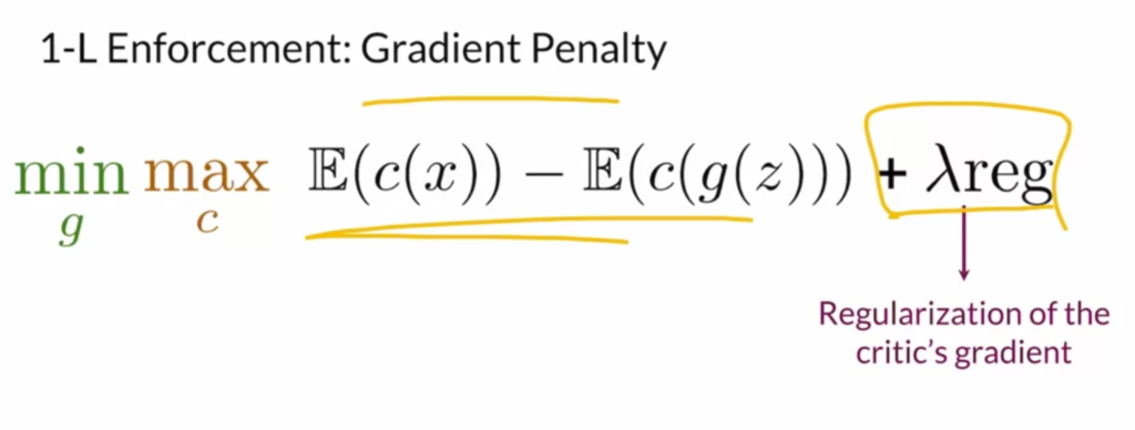
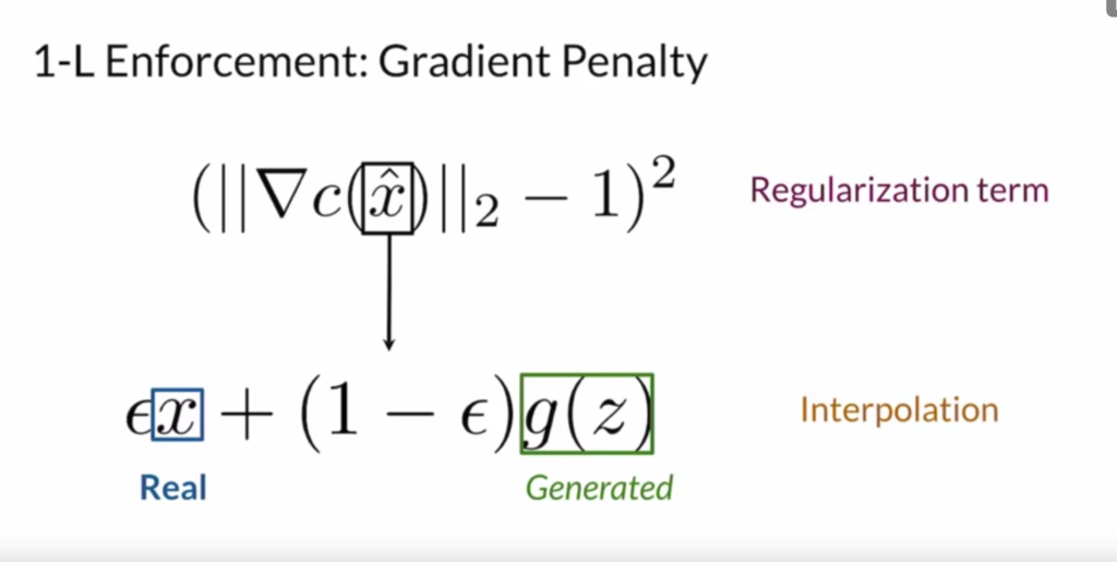
It is interesting to see that how 1-Lipschitz continuity (i.e., the gradient the discriminator/critic is no larger than 1) is soft-enforced by adding a penalty term.
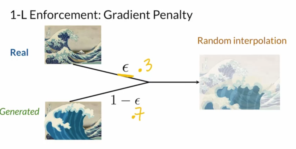
Instead of checking the critic is 1-Lipschitz continuity for every input, we sample an intermediate image by combining a real and fake image. We then encourage the gradient norm on the intermediate image to be within 1.
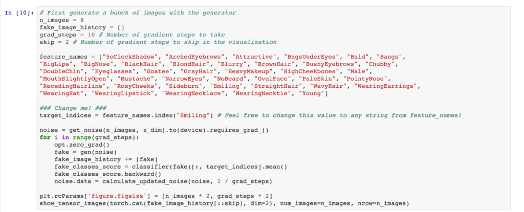
It is also intriguing to see how we can control GANs to generate images containing specific features. The first method is to utilize a pre-trained classifier, which scores how much a desired feature is present in a generated image.
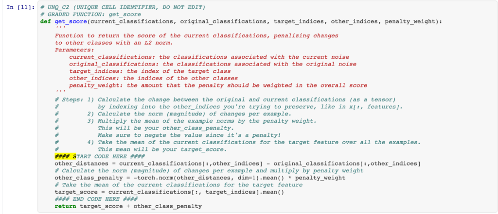
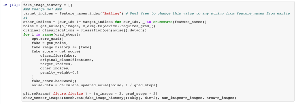
A slightly improved method is disentanglement, which makes sure other features do not change simultaneously.
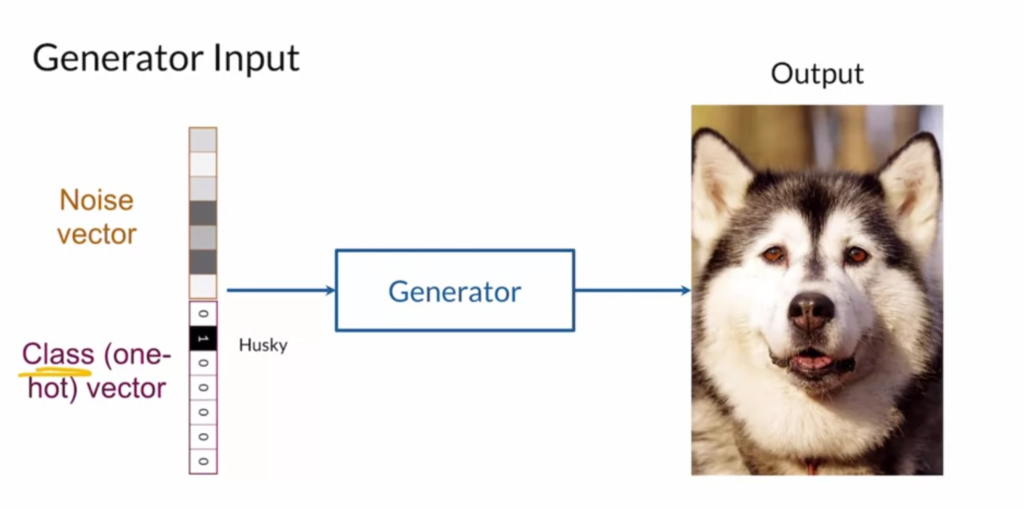
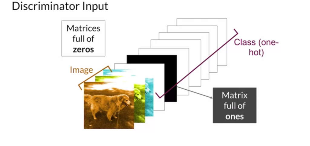
The second method is to augment the generator and discriminator’s input with a one-hot class vector. So you can ask the generator what class to generate, and you can ask the discriminator how relevant a generated image is to a given class, as shown below. Instead of requiring a pre-trained class as in the first method, the second method requires knowing the labels of training data.
The third method is infoGAN [5], which requires neither pre-trained models nor data labels. InfoGAN tries to learn latent codes that can control the output of the generator. The generator  takes as input a noise vector
  (as in the original GAN) and additionally, a latent code
  that learns semantic categories by unsupervised learning. A clever idea is proposed that the mutual information between
  and ,
and ,  should be maximized. In other words,
  should reveal as much information as possible about , which means we force the generator to generate images as much relevant to as possible. A similar idea is mentioned in our previous post when talking about the InfoNCE loss [6]. This notebook (C1W4_(Optional_Notebook)_InfoGAN) walks through the implementation of InfoGAN.
The lecture then moves on to evaluation metrics for GAN. One metric is based on Fréchet distance. We use some pre-trained image models such as Inception-v3 to process images and get embeddings, usually the output of one hidden layer. If we process N real images and N fake images, we would have N real images’ embeddings and N fake images’ embeddings. We can quantitatively compare the two embedding distributions by Fréchet distance, which has the following form:

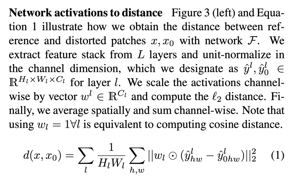
Another evaluation metric is from [7] called “Learned Perceptual Image Patch Similarity”. They also extract image features from  layers of a pre-trained network. As shown in Eqn. 1 below, the distance between two images is a weighted sum of per-layer similarity. There is a learnable parameter
  in per-layer similarity, which is learned to optimize for differentiating more similar image pairs from less similar pairs. Eventually, LPIPS can be used to measure the distance between real and fake images in GAN.

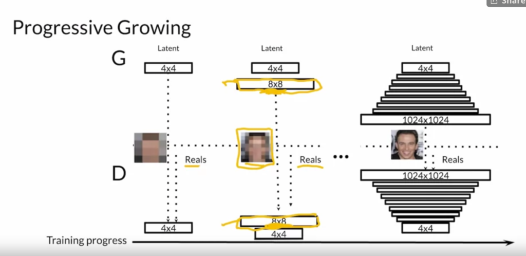
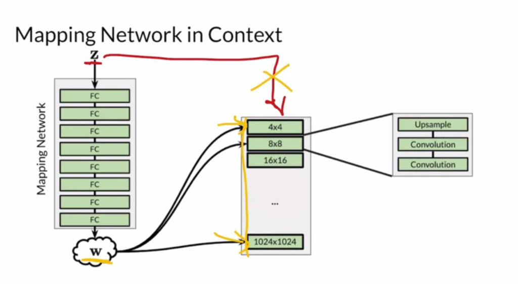
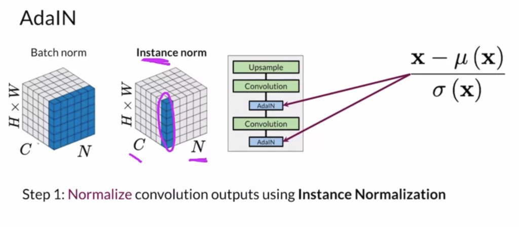
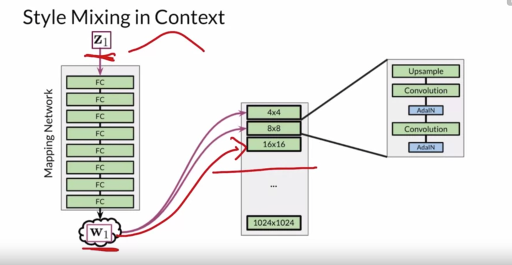
Finally, the lecture discusses one state-of-the-art GAN called StyleGAN [8]. There are three main components of StyleGAN: (1) progressive growing, (2) noise mapping network, and (3) adaptive instance normalization.

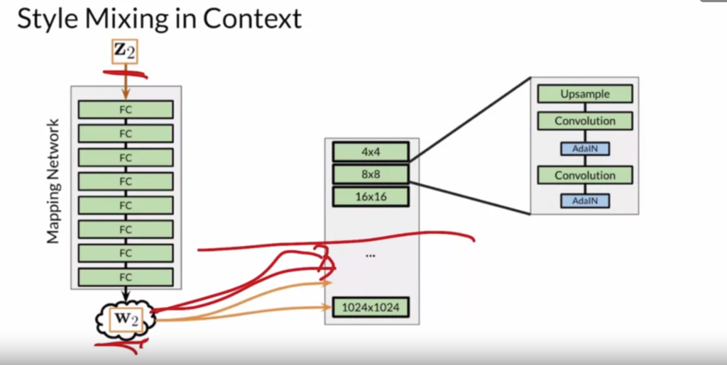
StyleGAN supports two ways of style variation. The first is styling mixing, which feeds different  vectors to different layers of the generator:
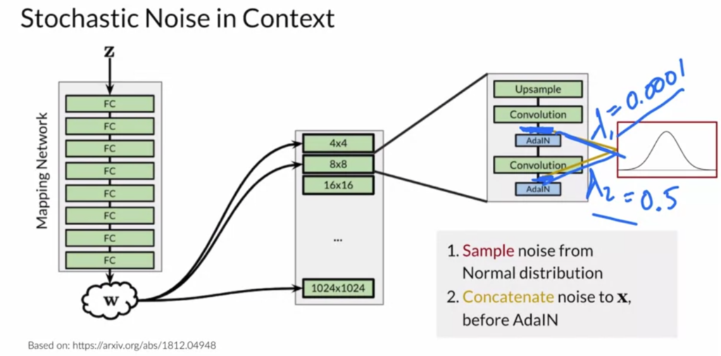
The second way to do style variation is to sample noise and add it between adaptive instance sampling operations.
References
[1] Unsupervised Representation Learning with Deep Convolutional Generative Adversarial Networks
[2] Up-sampling with Transposed Convolution
[3] https://arxiv.org/pdf/1701.07875.pdf
[4] https://zhuanlan.zhihu.com/p/25071913
[5] InfoGAN: Interpretable Representation Learning by Information Maximizing Generative Adversarial Nets
[6] Noise-Contrastive Estimation https://czxttkl.com/2020/07/30/noise-contrastive-estimation/
[7] The Unreasonable Effectiveness of Deep Features as a Perceptual Metric https://arxiv.org/pdf/1801.03924.pdf
[8] A Style-Based Generator Architecture for Generative Adversarial Networks https://arxiv.org/abs/1812.04948