Causal Inference

I’ve given a causal inference 101 in [7]. Since then I have been learning more and more about causal inference. I find Jonas Peters’ series of lectures quite good [1~4]. In this post, I am going to take some notes as I watch his lectures, and I am going to share some classic papers in causal inference.

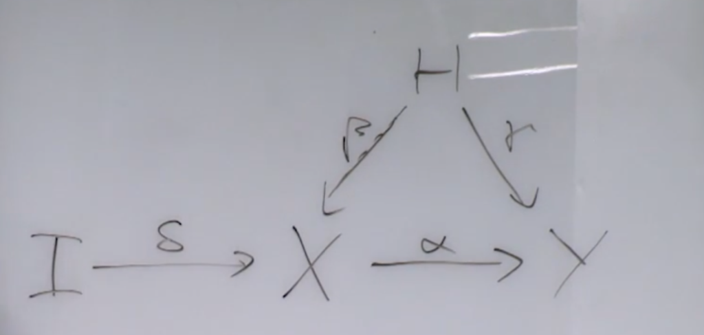
11:27 in [2], Jonas talked about two-stage regression. The problem is as follows. You want to know the causal effect of $X$ on $Y$ but there is some unobserved confounding factor that may impede your estimation (i.e., you can’t directly do $Y = \alpha X + N_y$ regression). So we can introduce an instrument variable $I$ which does not directly cause $Y$ by assumption. In the example he gave, $X$ is smoking, $Y$ is lung cancer, and $H$ is some hidden confounding factor that may affect $X$ and $Y$ , for example, stress level. $I$ is the tax on tobacco. By intuition, we assume the tax on tobacco doesn’t cause the change in stress level and lung cancer.

It must be a linear system for two-stage regression to work. We assume the underlying system can be described by the following linear equations:

$Y=\alpha X + \gamma H + N_y$
$X=\beta H + \sigma I + N_x$

Therefore, by replacing $X$ ‘s equation into $Y$ , we have:
$Y=(\alpha \beta + \gamma) H + \alpha \sigma I + \alpha N_x + N_y$

From the above equation, it becomes clear how to estimate $\alpha$ without depending on $H$ . First, we regress $X$ on $I$ , so that we can obtain $\sigma$ . Then using the fitted value of $X$ : $\hat{X}=\sigma I$ , we regress $Y$ on $\hat{X}$ . The coefficient learned that is associated with $\hat{X}$ would be roughly $\alpha$ , because the rest components $(\alpha \beta + \gamma) H + \alpha N_x + N_y$ in $Y$ is independent of $\sigma I$ .

However, this method would not work if the system is non-linear because then it is hard to separate $\sigma I$ from the rest components. $\alpha$ would be intertwined in different components which can’t be learned easily.

A real-world application of using two-stage regression is [5], where $X$ is time spent on different video types, $Y$ is overall user satisfaction, $H$ is some hidden user preference that may cause both users spending time on videos and their satisfaction. To really understand the magnitude of causal effect of video watch time and user satisfaction, they look at data from different online A/B test groups, with $I$ being a one-hot encoding of the test group a data belong to. Following the same procedure as two-stage regression, we can argue that $I$ does not cause either $Y$ or $H$ directly. The contribution of [5] is it reduces the bias when estimating the causal effect $\alpha$ .

28:00 in [2], Jonas introduced counterfactual distribution. He introduced an example which I think can best illustrate the difference between intervention distribution and counterfactual distribution. See their notations from “Notation and Terminology” in [6].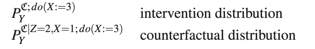

The example goes by follows.

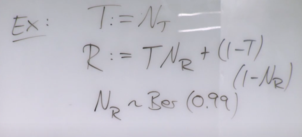
Suppose $T$ is a treatment to a disease. $R$ is the recovery result, which depends on whether one receives the treatment and a noise $N_R$ following a Bernoulli distribution. According to the provided structural causal model (SCM), the intervention distribution of $P_R(\text{do}(T:=1))$ would be $N_R$ . In natural language, a patient will have 0.99 probability to recover if received the treatment.

However, if we observed a specific patient who receives the treatment but did not recover, then we know this patient’s $N_R$ is sampled at value 0. So his counterfactual distribution if he were not received the treatment is $P_R(N_R=0;\text{do}(T:=0)) = 1$ . Note that this specific patient has a new SCM: $T= 1$ , $R=1-T$ . The counterfactual distribution $P_R(N_R=0;\text{do}(T:=0))$ on the old SCM would be the same as the intervention distribution on the new SCM.

I’ve talked about causal discovery using regression and noise independence test in [7]. Here is one another more example. In a CV paper [8], the authors want to determine the arrow of time given video frames. They model the time series’ next value as a linear function of the past two values plus additive independent noise. The final result shows that the forward-time series has a higher independence test p-value than the backward-time series. (A high p-value means we cannot reject the null hypothesis that the noise is independent of the input.) They only keep the data as valid time-series if the noise in the regression model for one direction at least is non-Gaussian, determined by a normality test. The noise independence test is “based on an estimate of the Hilbert-Schmidt norm of the cross-covariance operator between two reproducing kernel Hilbert spaces associated with the two variables whose in- dependence we are testing”.

Another interesting idea about causal discovery is causal invariant prediction. The goal of causal invariant prediction is to find all parents that cause a variable of interest $Y$ among all possible features $\{X_1, X_2, \cdots, X_p\}$ . The core assumption of causal invariant prediction is that in a SCM and any inventional distribution based on it, $P(Y|PA_Y)$ remains invariant if the structural equation for $Y$ does not change. Therefore based on data from different SCMs of the same set of variables (which can be observational data or interventional experiments), we can try to fit a linear regression $Y \leftarrow \sum\limits_{k\in S}\gamma_k X_k + \epsilon_Y$ for every feature subset $S \subset \{X_1, X_2, \cdots, X_p\}$ for each SCM. Across different SCMs, we would find all $S$ ‘s which lead to the same estimation of $\gamma_k, k \in S$ . 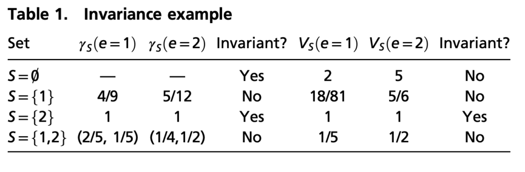Then the parent of $Y$ is the intersection of all the filtered $S$ ‘s because the interaction features’s relationship to $Y$ remains invariant all the time, satisfying our assumption of causal invariant prediction. [9] applies causal invariant prediction on gene perturbation experiments and I find the example in Table 1 is very illustrative.