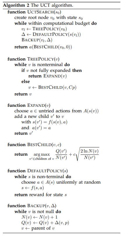
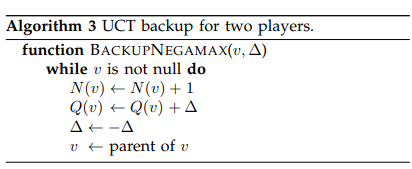
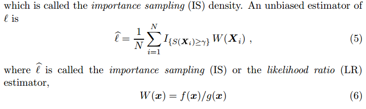
In this post, I am going to walk through an online piece of code [7] which implements the idea of [1]: using pointer network [2] to solve travelling salesman problem. Pointer networks, in my understanding, are neural network architectures for the problems where output sequences come from the permutation of input sequences.
Some background posts you may read in first:
[3]: policy gradient such as REINFORCE
[4]: LSTM code walk through
[5, 6]: travelling salesman problem
The code is based on [7] but modified in several small places to work with python 3.6 and torch 0.3.0 and cuda 8.0.
import math
import numpy as np
import torch
import torch.nn as nn
import torch.optim as optim
import torch.autograd as autograd
import torch.nn.functional as F
from torch.autograd import Variable
from torch.utils.data import Dataset, DataLoader
from IPython.display import clear_output
from tqdm import tqdm
import matplotlib.pyplot as plt
USE_CUDA = True
class TSPDataset(Dataset):
def __init__(self, num_nodes, num_samples, random_seed=111):
super(TSPDataset, self).__init__()
torch.manual_seed(random_seed)
self.data_set = []
for l in tqdm(range(num_samples)):
x = torch.FloatTensor(2, num_nodes).uniform_(0, 1)
self.data_set.append(x)
self.size = len(self.data_set)
def __len__(self):
return self.size
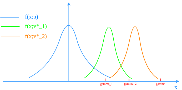
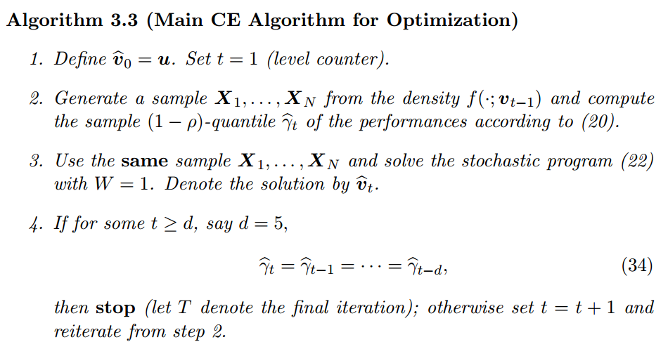
def __getitem__(self, idx):
return self.data_set[idx]
def reward(sample_solution):
"""
Args:
sample_solution seq_len of [batch_size]
"""
batch_size = sample_solution[0].size(0)
n = len(sample_solution)
tour_len = Variable(torch.zeros([batch_size]))
if USE_CUDA:
tour_len = tour_len.cuda()
for i in range(n - 1):
tour_len += torch.norm(sample_solution[i] - sample_solution[i + 1], dim=1)
tour_len += torch.norm(sample_solution[n - 1] - sample_solution[0], dim=1)
return tour_len
class Attention(nn.Module):
def __init__(self, hidden_size, use_tanh=False, C=10, name='Bahdanau'):
super(Attention, self).__init__()
self.use_tanh = use_tanh
self.C = C
self.name = name
if name == 'Bahdanau':
self.W_query = nn.Linear(hidden_size, hidden_size)
self.W_ref = nn.Conv1d(hidden_size, hidden_size, 1, 1)
V = torch.FloatTensor(hidden_size)
if USE_CUDA:
V = V.cuda()
self.V = nn.Parameter(V)
self.V.data.uniform_(-(1. / math.sqrt(hidden_size)), 1. / math.sqrt(hidden_size))
def forward(self, query, ref):
"""
Args:
query: [batch_size x hidden_size]
ref: ]batch_size x seq_len x hidden_size]
"""
batch_size = ref.size(0)
seq_len = ref.size(1)
if self.name == 'Bahdanau':
ref = ref.permute(0, 2, 1)
query = self.W_query(query).unsqueeze(2) # [batch_size x hidden_size x 1]
ref = self.W_ref(ref) # [batch_size x hidden_size x seq_len]
expanded_query = query.repeat(1, 1, seq_len) # [batch_size x hidden_size x seq_len]
V = self.V.unsqueeze(0).unsqueeze(0).repeat(batch_size, 1, 1) # [batch_size x 1 x hidden_size]
logits = torch.bmm(V, F.tanh(expanded_query + ref)).squeeze(1)
elif self.name == 'Dot':
query = query.unsqueeze(2)
logits = torch.bmm(ref, query).squeeze(2) # [batch_size x seq_len x 1]
ref = ref.permute(0, 2, 1)
else:
raise NotImplementedError
if self.use_tanh:
logits = self.C * F.tanh(logits)
else:
logits = logits
return ref, logits
class GraphEmbedding(nn.Module):
def __init__(self, input_size, embedding_size):
super(GraphEmbedding, self).__init__()
self.embedding_size = embedding_size
self.embedding = torch.FloatTensor(input_size, embedding_size)
if USE_CUDA:
self.embedding = self.embedding.cuda()
self.embedding = nn.Parameter(self.embedding)
self.embedding.data.uniform_(-(1. / math.sqrt(embedding_size)), 1. / math.sqrt(embedding_size))
def forward(self, inputs):
batch_size = inputs.size(0)
seq_len = inputs.size(2)
embedding = self.embedding.repeat(batch_size, 1, 1)
embedded = []
inputs = inputs.unsqueeze(1)
for i in range(seq_len):
a = torch.bmm(inputs[:, :, :, i].float(), embedding)
embedded.append(a)
embedded = torch.cat(embedded, 1)
return embedded
class PointerNet(nn.Module):
def __init__(self,
embedding_size,
hidden_size,
seq_len,
n_glimpses,
tanh_exploration,
use_tanh,
attention):
super(PointerNet, self).__init__()
self.embedding_size = embedding_size
self.hidden_size = hidden_size
self.n_glimpses = n_glimpses
self.seq_len = seq_len
self.embedding = GraphEmbedding(2, embedding_size)
self.encoder = nn.LSTM(embedding_size, hidden_size, batch_first=True)
self.decoder = nn.LSTM(embedding_size, hidden_size, batch_first=True)
self.pointer = Attention(hidden_size, use_tanh=use_tanh, C=tanh_exploration, name=attention)
self.glimpse = Attention(hidden_size, use_tanh=False, name=attention)
self.decoder_start_input = nn.Parameter(torch.FloatTensor(embedding_size))
self.decoder_start_input.data.uniform_(-(1. / math.sqrt(embedding_size)), 1. / math.sqrt(embedding_size))
def apply_mask_to_logits(self, logits, mask, idxs):
batch_size = logits.size(0)
clone_mask = mask.clone()
if idxs is not None:
clone_mask[[i for i in range(batch_size)], idxs.data] = 1
logits[clone_mask] = -np.inf
return logits, clone_mask
def forward(self, inputs):
"""
Args:
inputs: [batch_size x 2 x sourceL]
"""
batch_size = inputs.size(0)
seq_len = inputs.size(2)
assert seq_len == self.seq_len
embedded = self.embedding(inputs)
encoder_outputs, (hidden, context) = self.encoder(embedded)
prev_probs = []
prev_idxs = []
mask = torch.zeros(batch_size, seq_len).byte()
if USE_CUDA:
mask = mask.cuda()
idxs = None
decoder_input = self.decoder_start_input.unsqueeze(0).repeat(batch_size, 1)
for i in range(seq_len):
_, (hidden, context) = self.decoder(decoder_input.unsqueeze(1), (hidden, context))
query = hidden.squeeze(0)
for i in range(self.n_glimpses):
ref, logits = self.glimpse(query, encoder_outputs)
logits, mask = self.apply_mask_to_logits(logits, mask, idxs)
query = torch.bmm(ref, F.softmax(logits).unsqueeze(2)).squeeze(2)
_, logits = self.pointer(query, encoder_outputs)
logits, mask = self.apply_mask_to_logits(logits, mask, idxs)
probs = F.softmax(logits)
idxs = probs.multinomial().squeeze(1)
for old_idxs in prev_idxs:
if old_idxs.eq(idxs).data.any():
print(seq_len)
print(' RESAMPLE!')
idxs = probs.multinomial().squeeze(1)
break
decoder_input = embedded[[i for i in range(batch_size)], idxs.data, :]
prev_probs.append(probs)
prev_idxs.append(idxs)
return prev_probs, prev_idxs
class CombinatorialRL(nn.Module):
def __init__(self,
embedding_size,
hidden_size,
seq_len,
n_glimpses,
tanh_exploration,
use_tanh,
reward,
attention):
super(CombinatorialRL, self).__init__()
self.reward = reward
self.actor = PointerNet(
embedding_size,
hidden_size,
seq_len,
n_glimpses,
tanh_exploration,
use_tanh,
attention)
if USE_CUDA:
self.actor = self.actor.cuda()
def forward(self, inputs):
"""
Args:
inputs: [batch_size, input_size, seq_len]
"""
batch_size = inputs.size(0)
input_size = inputs.size(1)
seq_len = inputs.size(2)
probs, action_idxs = self.actor(inputs)
actions = []
inputs = inputs.transpose(1, 2)
for action_id in action_idxs:
actions.append(inputs[[x for x in range(batch_size)], action_id.data, :])
action_probs = []
for prob, action_id in zip(probs, action_idxs):
action_probs.append(prob[[x for x in range(batch_size)], action_id.data])
R = self.reward(actions)
return R, action_probs, actions, action_idxs
class TrainModel:
def __init__(self, model, train_dataset, val_dataset, batch_size=128, threshold=None, max_grad_norm=2.):
self.model = model
self.train_dataset = train_dataset
self.val_dataset = val_dataset
self.batch_size = batch_size
self.threshold = threshold
self.train_loader = DataLoader(train_dataset, batch_size=batch_size, shuffle=True, num_workers=1)
self.val_loader = DataLoader(val_dataset, batch_size=batch_size, shuffle=True, num_workers=1)
self.actor_optim = optim.Adam(model.actor.parameters(), lr=1e-4)
self.max_grad_norm = max_grad_norm
self.train_tour = []
self.val_tour = []
self.epochs = 0
def train_and_validate(self, n_epochs):
critic_exp_mvg_avg = torch.zeros(1)
if USE_CUDA:
critic_exp_mvg_avg = critic_exp_mvg_avg.cuda()
for epoch in range(n_epochs):
for batch_id, sample_batch in enumerate(self.train_loader):
self.model.train()
inputs = Variable(sample_batch)
if USE_CUDA:
inputs = inputs.cuda()
R, probs, actions, actions_idxs = self.model(inputs)
if batch_id == 0:
critic_exp_mvg_avg = R.mean()
else:
critic_exp_mvg_avg = (critic_exp_mvg_avg * beta) + ((1. - beta) * R.mean())
advantage = R - critic_exp_mvg_avg
logprobs = 0
for prob in probs:
logprob = torch.log(prob)
logprobs += logprob
logprobs[(logprobs < -1000).data] = 0.
reinforce = advantage * logprobs
actor_loss = reinforce.mean()
self.actor_optim.zero_grad()
actor_loss.backward()
torch.nn.utils.clip_grad_norm(self.model.actor.parameters(),
float(self.max_grad_norm), norm_type=2)
self.actor_optim.step()
# critic_exp_mvg_avg = critic_exp_mvg_avg.detach()
self.train_tour.append(R.mean().data[0])
if batch_id % 10 == 0:
self.plot(self.epochs)
if batch_id % 100 == 0:
self.model.eval()
for val_batch in self.val_loader:
inputs = Variable(val_batch)
if USE_CUDA:
inputs = inputs.cuda()
R, probs, actions, actions_idxs = self.model(inputs)
self.val_tour.append(R.mean().data[0])
if self.threshold and self.train_tour[-1] < self.threshold:
print("EARLY STOPPAGE!")
break
self.epochs += 1
def plot(self, epoch):
clear_output(True)
plt.figure(figsize=(20, 5))
plt.subplot(131)
plt.title('train tour length: epoch %s reward %s' % (
epoch, self.train_tour[-1] if len(self.train_tour) else 'collecting'))
plt.plot(self.train_tour)
plt.grid()
plt.subplot(132)
plt.title(
'val tour length: epoch %s reward %s' % (epoch, self.val_tour[-1] if len(self.val_tour) else 'collecting'))
plt.plot(self.val_tour)
plt.grid()
# plt.show()
plt.savefig('output.png')
print('train tour length: epoch %s reward %s' % (
epoch, self.train_tour[-1] if len(self.train_tour) else 'collecting'))
print(
'val tour length: epoch %s reward %s' % (epoch, self.val_tour[-1] if len(self.val_tour) else 'collecting'))
print('\n')
if __name__ == '__main__':
train_size = 1000000
val_size = 10000
seq_len = 20
train_20_dataset = TSPDataset(seq_len, train_size)
val_20_dataset = TSPDataset(seq_len, val_size)
embedding_size = 128
hidden_size = 128
batch_size = 64
n_glimpses = 1
tanh_exploration = 10
use_tanh = True
beta = 0.9
max_grad_norm = 2.
tsp_20_model = CombinatorialRL(
embedding_size,
hidden_size,
seq_len,
n_glimpses,
tanh_exploration,
use_tanh,
reward,
attention="Dot")
tsp_20_train = TrainModel(tsp_20_model,
train_20_dataset,
val_20_dataset,
threshold=3.99,
batch_size=batch_size)
tsp_20_train.train_and_validate(5)
Basically, we should start from line 368 where the main function starts. In this code, we focus on travelling salesman problems of size 20 on a 2D plane. That means, each data point of the training/validation dataset is a sequence of 20 2D points. Our goal is to search for a sequence of the given data points such that the loop trip for these data points has the shortest distance. Line 373 and 374 initialize the described datasets. In the following line (375 – 383), we set up model hyperparameters.
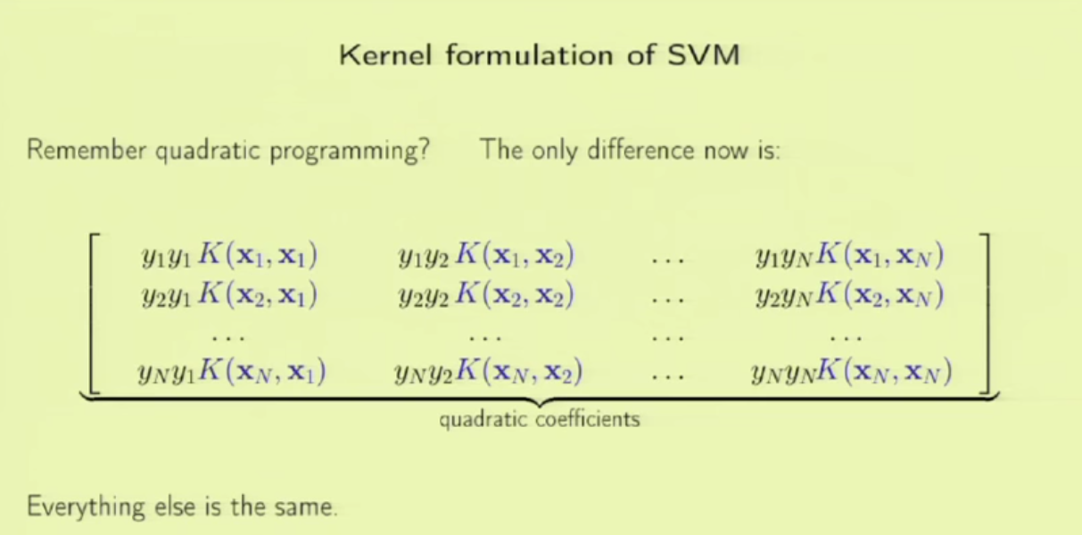
1. embedding_size is the dimension of transformed data from the original 2D data points. I think here the idea is to project 2D data into a higher dimension space such that richer information can be represented. It is possibly like devising a kernel in SVM [8] or like word embedding in NLP [9]. In line 173 (embedded = self.embedding(inputs) ), you can see that inputs to a pointer network must perform the embedding transformation first. (inputs size: batch_size x 2 x seq_len, embedded size: batch_size x seq_len x embedding_size)
2. n_glimpses is the number of glimpses to be performed in each decoder step (will explain more on it). However, since the author mentions in A.1 [1] that “We observed empirically that glimpsing more than once with the same parameters made the model less likely to learn and barely improved the results“, n_glimpses is simply set as 1.
3. tanh_exploration and use_tanh correspond to Eqn.16 in A.2 in [1], which is claimed to “help with exploration and yield marginal performance gains“.
We list the mapping between the paper parameters and the code parameters
| paper parameter |
note |
code parameter |
| $latex x$ |
input sequence of $latex n$ cities |
inputs |
| $latex \pi$ |
output sequence, permutation of $latex x$ |
actions |
| $latex n$ |
sequence length, the number of cities |
seq_len |
| $latex d$ |
the size of hidden units |
hidden_size |
| $latex B$ |
the size of Monte Carlo sampling for policy gradient |
batch_size |
| $latex k$ |
the number of encoder vectors to reference in attention/glimpse model. It is usually the same as $latex n$ |
|
After the last line calling tsp_20_train.train_and_validate(5) , we come into the real meat and potato (line 284 to line 344):
a. at line 293~295, we get a batch of inputs (inputs size: batch_size x 2 x seq_len)
b. at line 297 (R, probs, actions, actions_idxs = self.model(inputs) ), we pass inputs through a pointer network. We will talk about how the pointer network works. But for now, we just care about the workflow of TrainModel, which is essentially about training a policy gradient model called actor-critic.
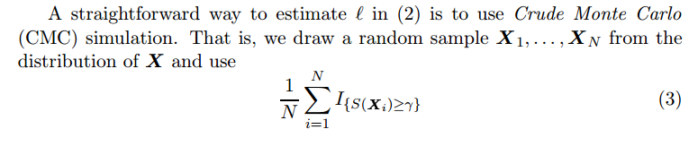
Policy gradient is a family of models in which the objective function is to directly optimize rewards generated according to a parameterized policy. More details can be found in [3]. The paper gives the formulation under REINFORCE algorithm [10]:


And the gradient of the policy (Eqn.4) can be approximated by the Monte Carlo method:
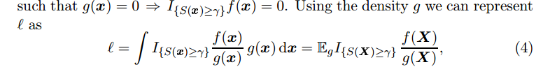
We can rewrite Eqn.5 to be more verbose, but more aligned to the codes:
$latex \nabla_\theta J(\theta) \approx \frac{1}{B}\sum\limits_{i=1}^B \nabla_\theta \sum\limits_{j=1}^n (L(\pi_i|s_i) – b(s_i)) \log p_\theta(\pi_i(j)|s_i) \;\; (5^*)&s=2$
Essentially, we expand $latex \log p_\theta(\pi_i | s_i)$ into $latex \sum\limits_{j=1}^n \log p_\theta(\pi_i(j) | s_i)$.
Since the learning framework like pytorch will compute the gradient automatically for us, we only need to compute $latex \frac{1}{B}\sum\limits_{i=1}^B \sum\limits_{j=1}^n (L(\pi_i|s_i) – b(s_i)) \log p_\theta(\pi_i(j)|s_i)&s=2$ using R and probs (line 306-320).
| parameter |
note |
size |
R |
rewards, $latex L(\pi_i|s_i)$ |
batch_size |
actions |
output data points |
seq_len x batch_size x 2 |
action_idxs |
output the order of input data points |
seq_len x batch_size |
probs |
the probability of each $latex p_\theta(\pi_i(j)|s_i)$ |
seq_len x batch_size |
Now, let’s transition to understand how the pointer network works (line 164-212). In line 174, self.encoder is a LSTM initiated at line 147. Since it is initialized with batch_first=True, embedded‘s size is batch_size x seq_len x embedding_size, with the batch_size as the first dimension. The output, encoder_outputs, also has the same size. (See [12] for pytorch I/O LSTM format.)
We are going to use the plot from the paper to further illustrate how the pointer network works. First, let’s get clear about where encoder_inputs (embedded) and encoder_outputs are.
Each blue block is the LSTM unit which takes input repeatedly. Since in line 174, self.encoder is fed without hidden and context parameter, hidden and context for the first input are treated as zero vectors [12]. LSTM will output, besides encoder_outputs, hidden and context layers:
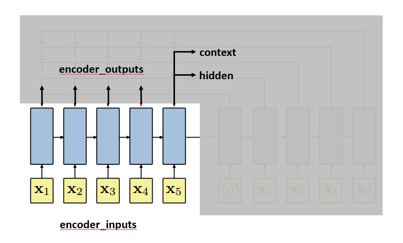
After the last input passes the encoder, the decoder will start. The first input to the decoder, denoted by <g>, is a vector of the same embedding size as the inputs. And it is treated as a trainable parameter. The first hidden and context vectors to the decoder are the last hidden and context vectors of the encoder. The decoder will output context and hidden vectors at each step.
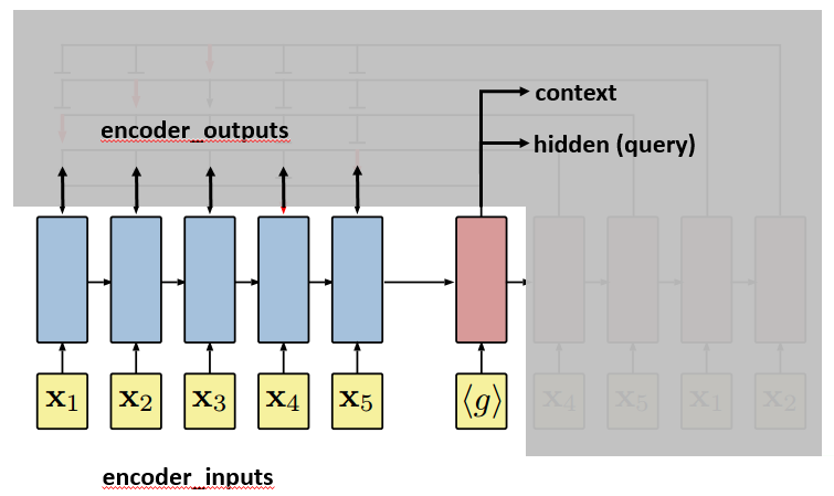
The hidden vector of the decoder, together with encoder_outputs, will be used by an attention model to select an output (city) at each step. Before hidden is sent to the attention model, the paper suggests to process it by a technique called “glimpse”. The basic idea is to not use hidden directly in the attention model, but use query=glimpse(hidden, encoder_outputs) $latex \in \mathbb{R}^d$. Te author says that “The glimpse function G essentially computes a linear combination of the reference vectors weighted by the attention probabilities“. Note the two things:
- the attention model to select output cities and the glimpse model are both attention models. The difference between the two is that the glimpse model outputs a vector with $latex d$ dimension to replace the hidden vector of the decoder while the attention model to select output cities outputs a vector with $latex k$ dimension, which refers to the probability distribution of selecting each of the $latex k$ reference vectors.
- Due to the nature of the problem, there cannot be duplicate cities in the output sequence. Therefore we have to manually disable those already outputted cities using the function
apply_mask_to_logits.
Finally, it comes to the attention model. The attention model will take as input the query vector and encoder_outputs. As we said, the attention model will output a probability distribution of length $latex k$, the number of reference vectors. $latex k$ is usually equal to $latex n$ because we reference all the input cities.
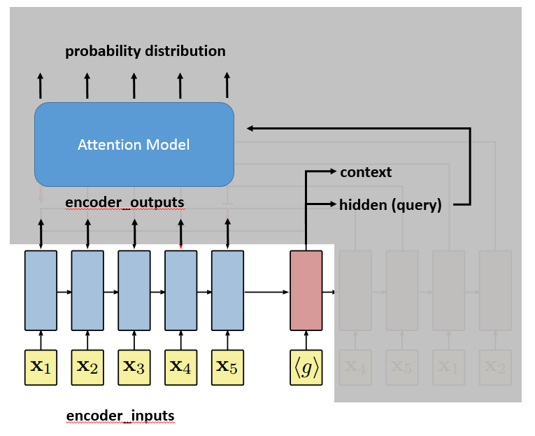
Line 200~206 finally selects the output city according to the probability distribution.
In line 207, we prepare the next input to the decoder, which is the embedding of the city just outputted.
The following table lists the sizes of all appeared parameters.
| parameter |
size |
embedded |
batch_size x seq_len x embedding_size |
encoder_outputs |
batch_size x seq_len x hidden_size |
hidden |
1 x batch_size x hidden_size |
context |
1 x batch_size x hidden_size |
query |
batch_size x hidden_size |
logits |
batch_size x seq_len |
Let’s pretty much about it.
Reference:
[1] Neural Combinatorial Optimization With Reinforcement Learning: https://arxiv.org/abs/1611.09940
[2] Pointer Networks: https://arxiv.org/abs/1506.03134
[3] https://czxttkl.com/?p=2812
[4] https://czxttkl.com/?p=1819
[5] https://czxttkl.com/?p=1047
[6] https://czxttkl.com/?p=3109
[7] https://github.com/higgsfield/np-hard-deep-reinforcement-learning
[8] https://czxttkl.com/?p=3114
[9] https://czxttkl.com/?p=2530
[10] Simple Statistical Gradient-Following Algorithms for Connectionist Reinforcement Learning: http://www-anw.cs.umass.edu/~barto/courses/cs687/williams92simple.pdf
[12] http://pytorch.org/docs/master/nn.html#torch.nn.LSTM


 . This is a straightforward, as its input is the board state
  (plus some move history and human engineered features) and its output is the action
  to take. The training data is essentially state-action pairs
  sampled from real human play matches. The goal of this supervised learning policy network is to accurately predict moves. Therefore, it is designed with convoluted structures with 13 layers. As reported, it can achieve 55.7% accuracy and takes 3ms per prediction.
 , which results in simpler structure, faster prediction time but less accuracy. It requires 2us per prediction and has 24.2% accuracy reportedly.
 trained based on the supervised learning policy network
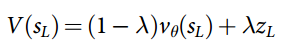
  which estimates the expected outcome from position
 ![v^{p_{\rho}}(s) = \mathbb{E}[z_t | s_t=s, a_{t \cdots T} \sim p_{\rho}]](https://czxttkl.com/wp-content/ql-cache/quicklatex.com-c4da6eea96d7f4fed2f05c7f1b9395c7_l3.png "Rendered by QuickLaTeX.com") . As the paper [1] stated, the most useful value network should estimate the expected outcome under perfect play,
. As the paper [1] stated, the most useful value network should estimate the expected outcome under perfect play,  , which means each of the two players acts optimally to maximize his own winning probability. But since we do not have perfect play as ground truth, we have to use
  . But note that, training a value network is not the only way to estimate
  . We can also use Monte Carlo rollouts to simulate a large number games by using
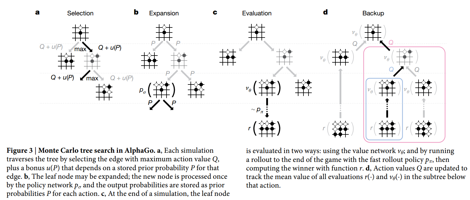
 and
and  :
: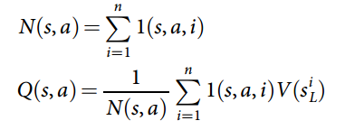
 is the value of the leaf state after the selection phase in simulation
  .
.  and a roll out outcome
  using the fast policy network
  :
:
 during the selection phase of a simulation, an action
  is selected according to:
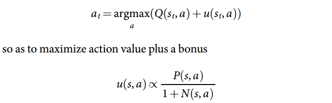
 ,
,  , and
, and  .
. which learns to output two heads: (1) an action probability distribution (
 , a vector, whose component is
  ); (2) and outcome value prediction (
 , a scalar).
 . At each move, an MCTS search is executed based on
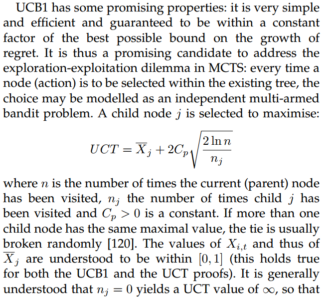
  in the simulation phase. The output of the MCTS search is an action distribution
  determined by the upper confidence bound for each action:
  where
where  , the same bound metric as in AlphaGo [1].
 . These distribution-outcome tuples will serve as the training data for updating the weights of
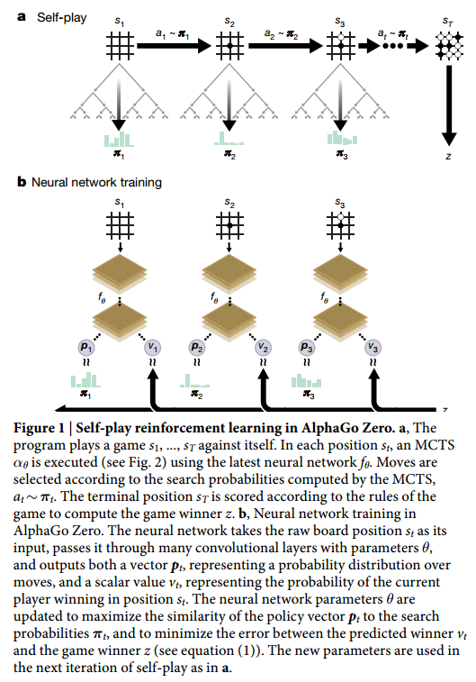
 , we could imagine that at some point each terminal state has been visited once:

 , where each point is a
  -dimensional data point
  associated with label
  .
. such that data points can be perfectly linearly divided according to their labels. For a linearly separable dataset, there can exist infinite such plane. However, the “best” one, intuitively, should have the largest margins from all the closest points to it. Here, “margin” means the distance from a point to a plane. As an example below, the best separating plane is supposed to be the rightmost one.
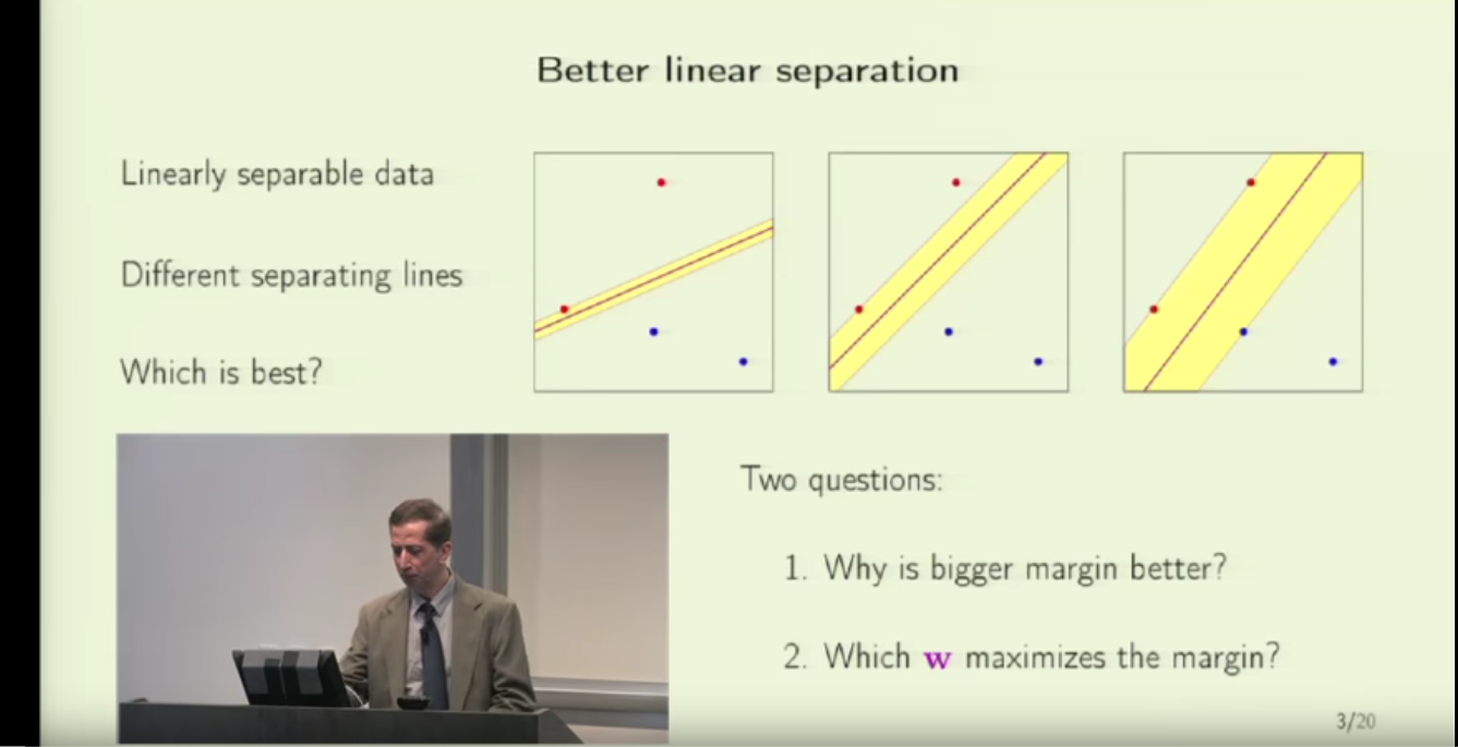
 , the way to calculate its margin (i.e., its distance to the plane
  , is to pick a point
  on the plane and then project
  onto
onto  :
: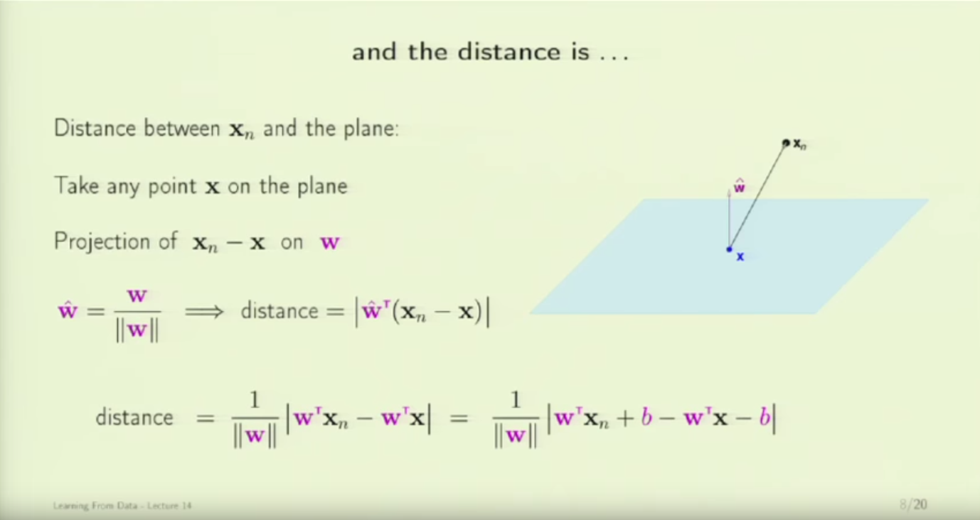

 . Therefore the distance from
 corresponding to it, all with different scales. For example, the plane
  with
with  is the same plane as the plane
  with
with  . Therefore, we need to pre-define a scale.
 such that the closest data point to the plane,
  . Therefore, the distance from the closest data point to the plane becomes
  . After this, the objective function becomes easier:
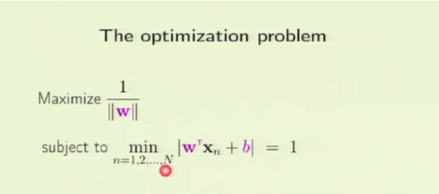
 . The constraints
  can be re-written as
  . Moreover, instead of maximizing
  equivalently. Therefore, the objective function now becomes:
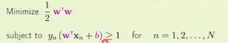
 ). That is the data point which is the closest to the plane. If all the constraints only have the inequality hold (i.e.,
  ),
),  decreases until some constraint hits the equality.
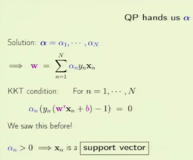
 ), KKT condition becomes a sufficient and necessary condition for finding the optimal solution
  .
.  (the Lagranger multipler),
  , and
, and 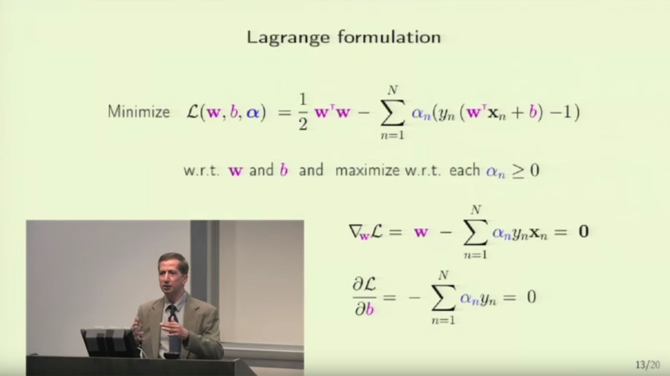
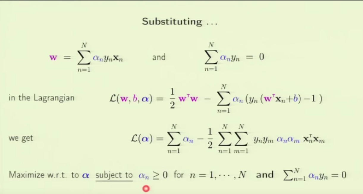
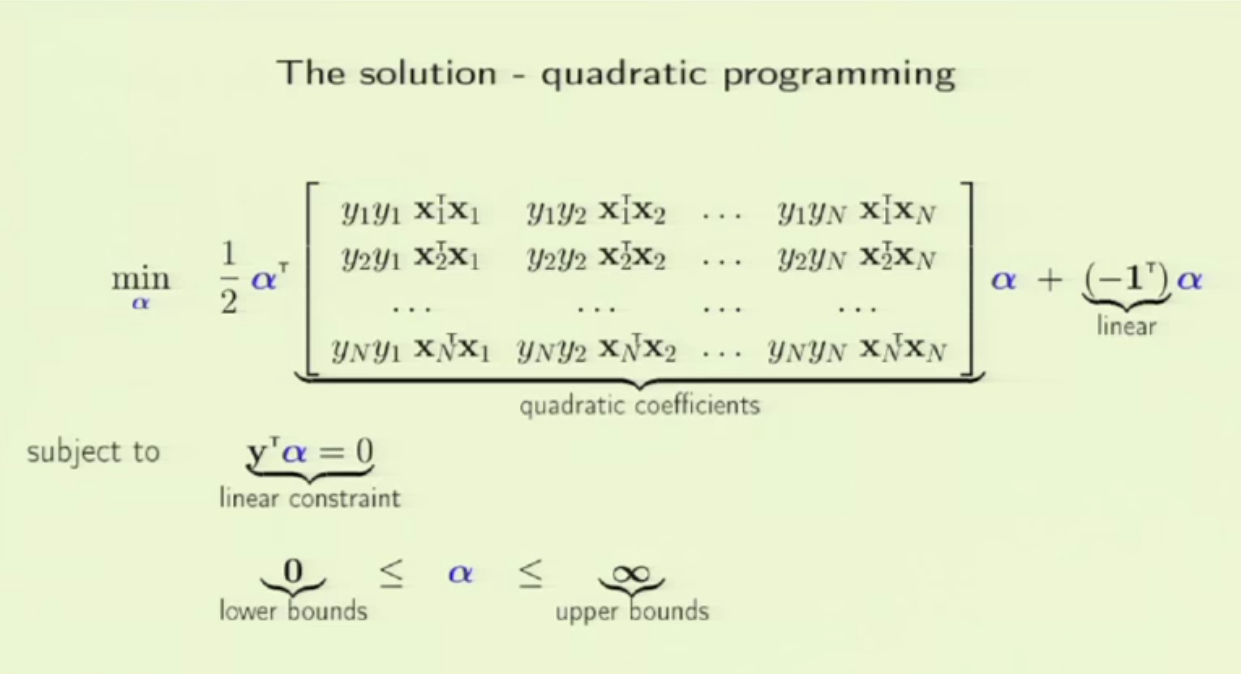
 .
. , which only requires we know the inner product between any
  . Suppose in the original form of raw data,
  are low-dimensional data points that are not linearly separable. However, if they are mapped to a higher dimension as
  , they can be separable. On that high dimension space, we can apply the linear separable SVM version on the data points
  and
and  .
.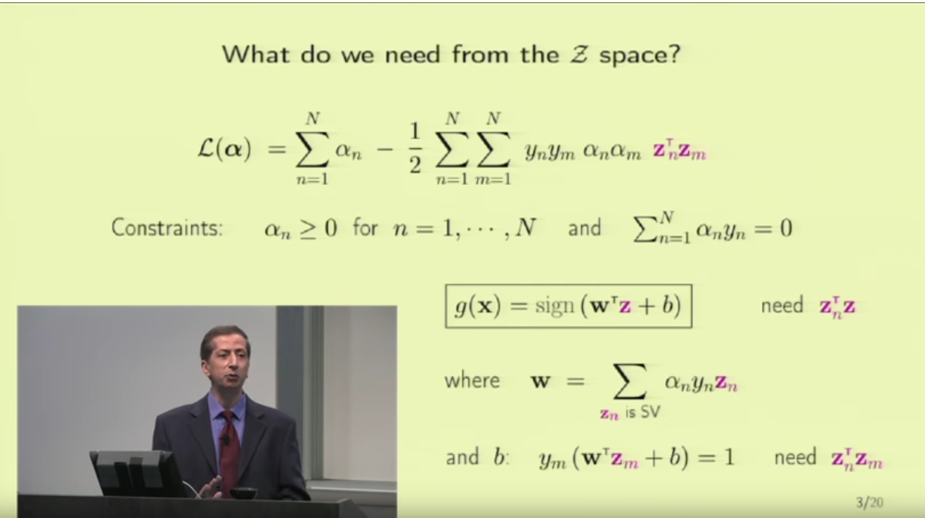
 : even a black-box mapping function is ok, as long as we can calculate the inner product of any
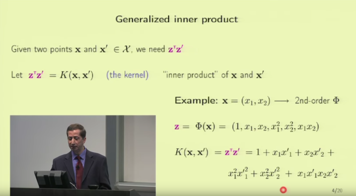
 and Radial Basis Function kernel:
  . There is a math property called “Mercer’s condition” that an be used to verify whether a function is a valid kernel function. But this is out of the scope of this post.