My understanding in Cross Entropy Method

Cross Entropy (CE) method is a general Monte Carlo method originally proposed to estimate rare-event probabilities but then naturally extended to solve optimization problems. It is relevant to several my previous posts. For example, both Bayesian Optimization [5] and CE method can be used to solve black-box optimization problems, although Bayesian Optimization mostly works on continuous input domains whereas CE mostly works on combinatorial black-box optimization problems, i.e., inputs are discrete. For another example, CE is largely based on importance sampling [1], a variance reduction method whose core idea is, when estimating the expectation of some quantity, sampling its random variables on a different pdf such that the variance of the estimation can be smaller than sampling on the original pdf [6].

In this post, I am going to talk about my understanding in CE method. My understanding largely comes from a great tutorial [2].

Let’s first see how CE works on rare-event probability evaluation. The goal of rare-event probability evaluation is to estimate:

$latex \ell=P(S(\textbf{X}) \geq \gamma) = \mathbb{E} \textit{I}_{\{S(\textbf{X}) \geq \gamma\}},&s=2$

where $latex \textbf{X}$ is a multidimensional random variable vector following a probability density function (pdf) $latex f(\textbf{x};\textbf{u})$, $latex S(\textbf{X})$ is a (possibly black-box) function that returns a quantity for any given $latex \textbf{X}$, $latex \textit{I}(\cdot)$ is an identity function returns 1 if what is inside is true otherwise 0.

[2] notes that the naive way to estimate $latex \ell$ is to use Crude Monte Carlo (CMC) simulation:

Screenshot from 2018-02-18 00-11-25

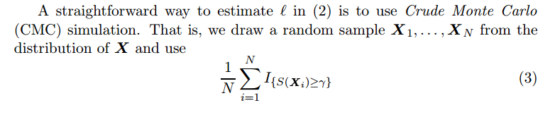
The disadvantage is that if $latex S(\textbf{X}) \geq \gamma$ is rare, in other word, $latex \gamma$ is large, positive samples will be scarce. Therefore, CMC may need a lot of time and samples before it returns a reliable estimation.

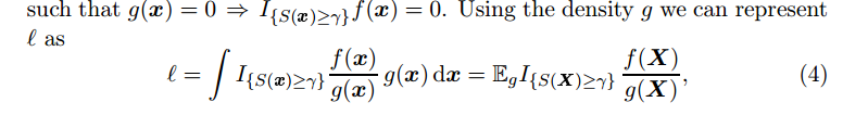
Therefore, we turn to another technique called importance sampling. In importance sampling, we sample $latex \textbf{X}$ in another distribution $latex g(\textbf{X})$, let’s say $latex g(\textbf{x})=f(\textbf{x}; \textbf{v})$, the same distribution family as $latex f(\textbf{x}; \textbf{u})$ but with different parameters. This converts estimating the expectation of $latex \textit{I}_{\{ S(\textbf{X}) \geq \gamma \}} &s=2$ to estimating the expectation of $latex \textit{I}_{\{ S(\textbf{X})\geq \gamma \}} \frac{f(\textbf{X})}{g(\textbf{X})} &s=2$:

Screenshot from 2018-02-18 00-33-18

Screenshot from 2018-02-18 00-34-13

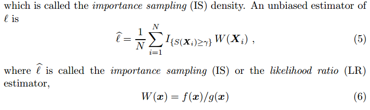
The central idea of importance sampling is that if sampling on $latex g(\textbf{x})=f(\textbf{x}; \textbf{v})$ can make the event $latex S(\textbf{X}) \geq \gamma$ appear more often, and if we know the exact form of $latex g(\textbf{x})$, and provided that we already know the exact form of $latex f(\textbf{x}; \textbf{u})$, then $latex \hat{\ell}$ (Eqn.5) would have smaller variance than Eqn. 3. In other words, we could have needed less samples to estimate $latex \ell$ in the same precision as in CMC.

In theory, the best $latex g(\textbf{x})$ from the same distribution family of $latex f(\textbf{x};\textbf{u})$ to reduce the estimation variance is:

Screenshot from 2018-02-18 12-22-08

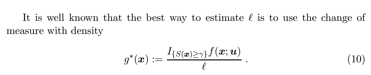
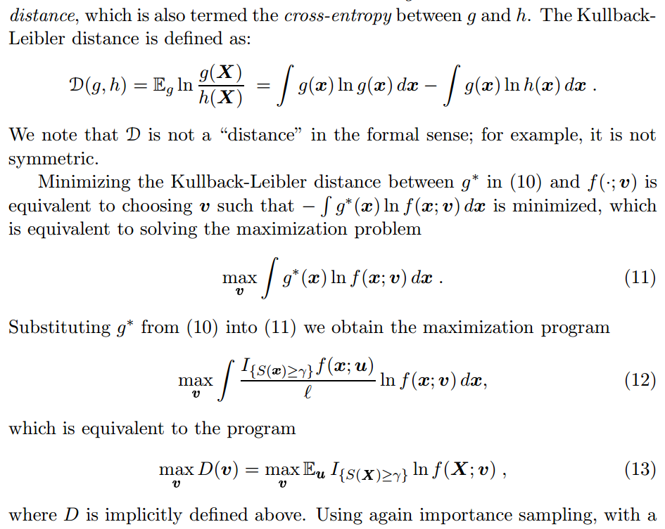
The obvious difficulty is that we do not know $latex g^*(\textbf{x})$ in advance because we do not know $latex \ell$ in advance. To tackle this, we want to fit a distribution from the same distribution family of $latex f(\textbf{x};\textbf{u})$ as close as possible to approximate $latex g^*(\textbf{x})$. This is achieved by searching for a set of parameters $latex \textbf{v}$ such that the Kullback-Leibler distance (also named cross-entropy) between $latex g^*(\textbf{x})$ and $latex f(\textbf{x};\textbf{v})$ is minimized:

Screenshot from 2018-02-18 12-33-45

To estimate Eqn. 13 stochastically, we have:

$latex \max_{\textbf{v}} D(\textbf{v}) = \max_{\textbf{v}} \frac{1}{N} \sum\limits_{i=1}^N \textit{I}_{\{S(\textbf{X}_i) \geq \gamma \}} ln(\textbf{X}_i;\textbf{v}) &s=2$,

where $latex \textbf{X}$ is drawn from $latex f(\textbf{x};\textbf{u})$.

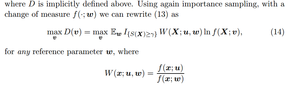
To this point, we still face the difficulty that the event $latex S(\textbf{X}) \geq \gamma$ happens rarely such that this estimation may have large variance. Therefore, we use importance sampling again and introduce another distribution $latex f(\textbf{x};\textbf{w})$ on Eqn. 13, hoping that $latex f(\textbf{x};\textbf{w})$ can make $latex S(\textbf{X}) \geq \gamma$ appear more often:

Screenshot from 2018-02-18 12-47-46

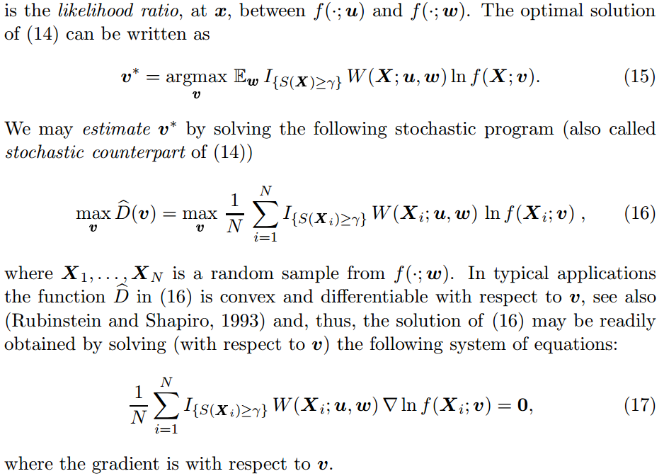
Now, the most important question is: how can we know $latex \textbf{w}$? After all, if we know $latex \textbf{w}$, the rest of the problem would be just to sample $latex \textbf{X}$ based on $latex f(\textbf{x};\textbf{w})$, and solve Eqn. 15 using Eqn. 16 and Eqn. 17.

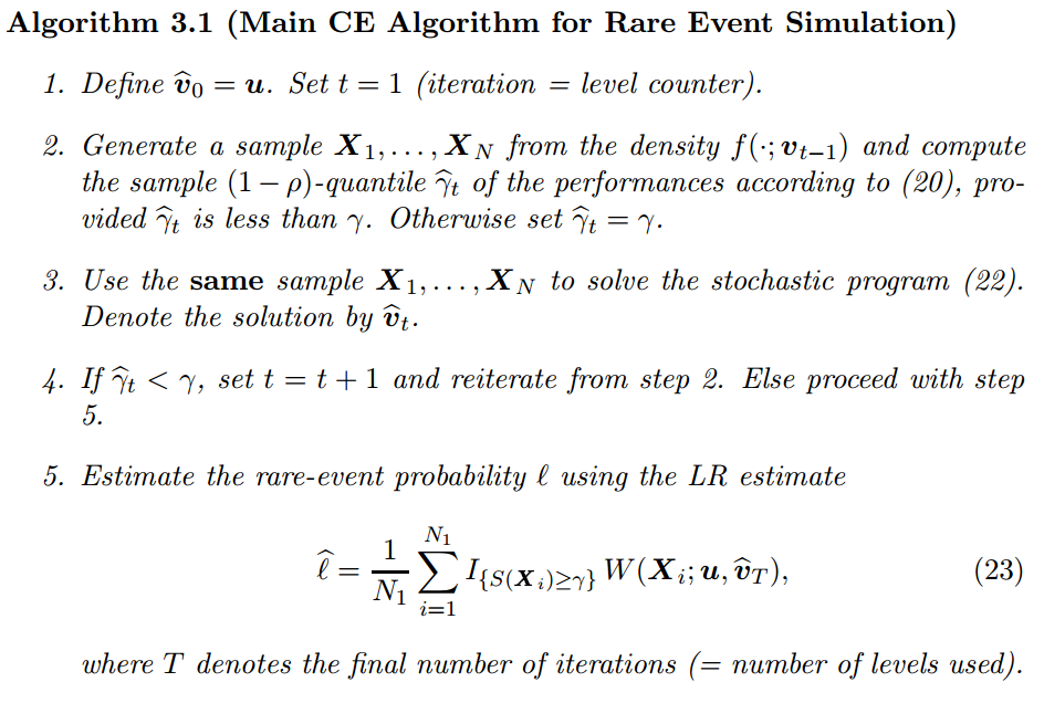
The answer is: we can obtain $latex \textbf{w}$ iteratively. We will also need a sequence $latex \{\gamma_t, t \geq 1\}$. We will start with $latex \textbf{w}_0=\textbf{u}$ and $latex \gamma_1 < \gamma$ such that $latex S(\textbf{X}) \geq \gamma_1$ isn’t too rare if sampling on $latex \textbf{w}_0$. A canonical way is to set $latex \rho=0.01$ and let $latex \gamma_1$ be the $latex (1-\rho)$-quantile of $latex S(X)$ sampling from $latex \textbf{w}_0$. Setting $latex \gamma=\gamma_1$ and $latex \textbf{w}=\textbf{w}_0$ in Eqn. 15, we can obtain $latex \textbf{v}^*_1$. You can think $latex f(\textbf{x}; \textbf{v}^*_1)$ the best distribution to sample for estimating $latex \mathbb{E}_{\textbf{u}} \textit{I}_{\{S(\textbf{X}) \geq \gamma_1 \}} $. More importantly, compared to $latex f(\textbf{x}; \textbf{u})$, sampling from $latex f(\textbf{x};\textbf{v}^*_1)$ makes the event $latex S(\textbf{X}) \geq \gamma$ a little less rare: the probability mass shifts a bit towards the event $latex S(\textbf{X}) \geq \gamma$.

The iteration goes on by setting $latex \textbf{w}_1=\textbf{v}^*_1$ and $latex \gamma_2$ to be the $latex (1-\rho)$-quantile of $latex S(X)$ sampling from $latex \textbf{w}_1$. Solving Eqn.15 can result to the best distribution $latex f(\textbf{x};\textbf{v}^*_2)$ to sample for estimating $latex \mathbb{E}_{\textbf{u}} \textit{I}_{\{S(\textbf{X}) \geq \gamma_2 \}}$. Again, the probability mass of $latex f(\textbf{x};\textbf{v}^*_2)$ shifts a little bit towards the event $latex S(\textbf{X}) \geq \gamma$.

The iterations loop until $latex \gamma_t$ is not less than $latex \gamma$, i.e., sampling $latex \textbf{X}$ from $latex \textbf{w}_t$ sees the event $latex S(\textbf{X}) \geq \gamma$ frequently enough. Until this point, Eqn. 5 can be used reliably to estimate $latex \ell$.

The full version of the algorithm is as follows:

Screenshot from 2018-02-18 14-09-46

I found it is useful to understand the whole process by using a toy example: $latex \textbf{X}$ is a one-dimension random variable. $latex S(\textbf{X})=\textbf{X}$. $latex f(\textbf{x};\textbf{u})$ is a just a normal distribution. $latex \gamma$ is a relatively large number falling outside the 3 times of the standard deviation of $latex f(\textbf{x};\textbf{u})$.

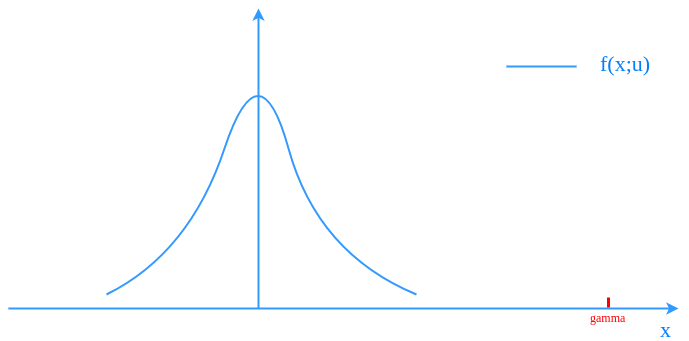
Obviously, sampling from $latex f(\textbf{x};\textbf{u})$ to estimate $latex \mathbb{E} \textit{I}_{\{S(\textbf{X}) \geq \gamma \}}$ requires a large number of samples. Following Algorithm 3.1, we will set a less rare $latex \gamma_1 < \gamma$ and calculate $latex f(\textbf{x};\textbf{v}^*_1)$.

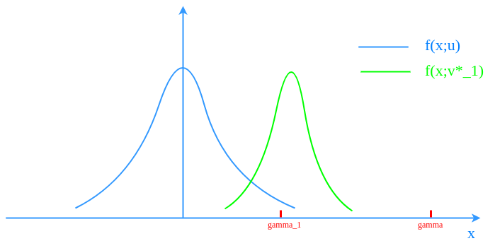
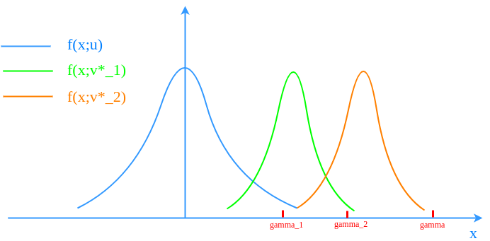
Keeping doing that will end up with $latex \gamma_t$ and $latex f(\textbf{x};\textbf{v}^*_t)$ shifting closer and closer to $latex \gamma$ until sampling $latex S(\textbf{X}) \geq \gamma$ is no longer too rare under $latex f(\textbf{x};\textbf{v}^*_t)$.

To this point, we finish introducing how CE method is applied in rare event probability estimation. Now, we introduce how CE method can be applied in combinatorial search problem. The setting of a typical combinatorial search problem is:

Screenshot from 2018-02-18 19-10-13

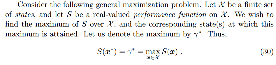
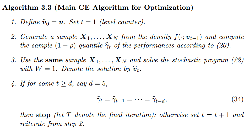
For every combinatorial search problem, we can associate it with a rare-event probability estimation problem: to estimate $latex P_{\textbf{u}}(S(\textbf{X}) \geq \gamma)$. It doesn’t matter how you choose the distribution $latex f(\textbf{x};\textbf{u})$ and $latex \gamma$ for the associated problem, what it matters is the pattern we observe in Algorithm 3.1: both intermediate distribution $latex f(\textbf{x};\textbf{v}^*_t)$ and $latex \gamma_t$ will iteratively shift towards the direction of the maximum of $latex S(\textbf{X})$. If we let the iteration loop long enough, $latex f(\textbf{x};\textbf{v}^*_t)$ and $latex \gamma_t$ will end up around the area of the maximum of $latex S(\textbf{X})$. After that, $latex \gamma_T$ will faithfully be close to $latex \gamma^*$ and sampling from $latex f(\textbf{x};\textbf{v}^*_T)$ will faithfully generate approximated optimal solution. This idea basically shapes Algorithm 3.3:

Screenshot from 2018-02-18 19-36-16