LambdaMART [7] is one of Learn to Rank algorithms. It emphasizes on fitting on the correct order of a list, which contains all documents returned by a query and marked as different relevance. It is a derivation/combination of RankNet, LambdaRank and MART (Multiple Addictive Regression Tree).
For me, the most helpful order to approach LambdaMART is to understand: 1. MART; 2. RankNet; 3. LambdaRank; and 4. LambdaMART. [4] actually aligns with my order to introduce LambdaMART. (Sidenote: another good resource to learn MART is [8])
1. MART
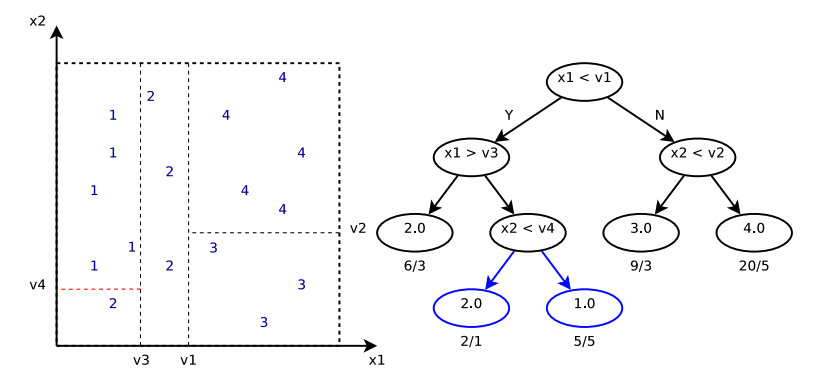
Above is an illustration plot for one regression tree. If data of different labels actually come from disjoint feature spaces, then one regression tree would be enough. However, there are many situations where data do come from interleaved feature spaces. Hence, it is natural to propose using multiple regression trees to differentiate irregular feature subspaces and make predictions.
Now, suppose MART’s prediction function is  , where each
  is one regression tree’s output and
  are the parameters of that tree. Generally speaking, each regression tree has K-terminal nodes. Hence contains
  , which are the K feature subspaces that divide data, and
  , which are the predicted outputs of data belonging to . can be represented as:
 are iteratively learned to fit to the training data:
- Set
 to initial guess
 - for each
 , we learn optimal feature space divisions
- Based on the learned, the prediction value of each
 (leaf) is deterministically fixed as:
Although [4] doesn’t provide details for learning , I guess they should be very similar to what adopted in normal decision trees. One possible criteria could be to minimize the total loss:  . (If using this criteria, and are actually learned simultaneously)
[4] provides an example to illustrate the iterative learning process. The dataset contains data points in 2 dimensions and labels  . The loss function
  is least square loss. Each regression tree is only a decision stump.
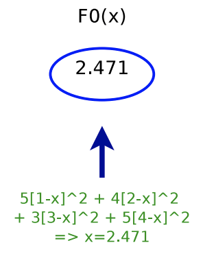
 is the simplest predictor that predicts a constant value minimizing the error for all training data.
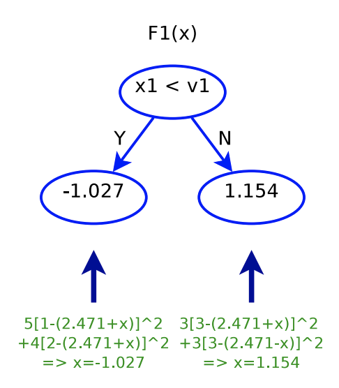
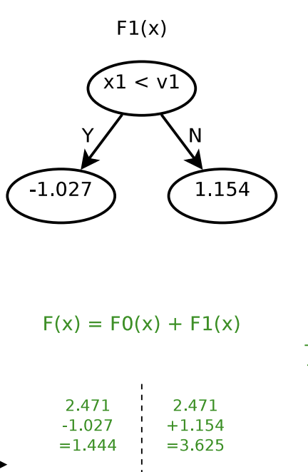
After determining  , we start to build
  . The cut
  is determined by some criterion not mentioned. But assuming that has already been obtained, we can then determine each leaf’s prediction output, i.e.,
  :
:
After determining the first and second trees,  . In other words, for
  , the predicted value will be 1.444; for
  , the predicted value will be 3.625.
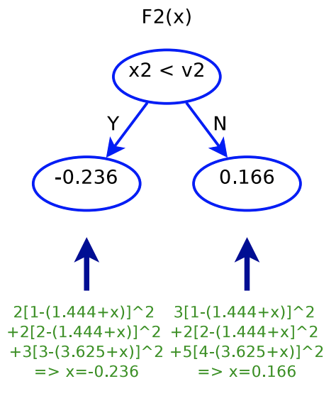
Next, determining  will be similar: finding a cut
  , and then determine
  as in step 3.
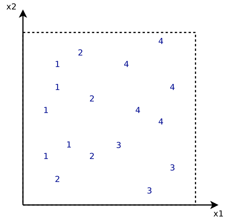
Interestingly, when we fit , it looks like that we fit a tree with each data point’s label updated as  , that is, we are fitting the residual of what previous trees are not able to predict. Below is the plot showing each data point’s original label and its updated label before fitting .
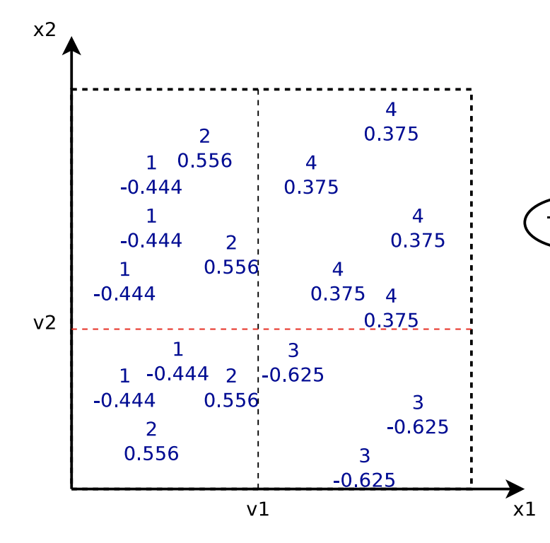
In fact, the fitting process described above is based on the assumption that  is a square loss function. When fitting the
  -th tree, we are fitting the tree to the residual
  . Interestingly,
  . That’s why MART is also called Gradient Boosted Decision Tree because that each tree fits the gradient of the loss.
To be more general and mathematical, when we learn and in the -th iteration, our objective function is:

If we take Taylor series of the objective function up to order 2 at 0, we get [10]:

Each time, the new regression tree ( and ) should minimize this objective function, which is a quadratic function with regard to
  . As long as we know
  and
and  , we can learn the best to minimize the objective function.
Now, back to the previous example, if is a square loss function  , then
  and
and  . Thus, the objective function becomes:

This is not different than  . That’s why in the above fitting process, it seems like we are fitting each new tree to the residual between the real label and previous trees’ output. In another equivalent perspective, we are fitting each new tree to the gradient
  .
.
The loss function can take many kinds of forms, making MART a general supervised learning model. When MART is applied on classification problems, then the loss function for each data point  is
is ![L(y_i, p_i)=- [y_i \log (p_i) + (1-y_i) \log (1-p_i)]](https://czxttkl.com/wp-content/ql-cache/quicklatex.com-e6faa5e549756e8e5ea8b26785a666f4_l3.png "Rendered by QuickLaTeX.com") , where
, where  is the predicted probability
  . The regression trees’ output is used to fit the logit of , i.e.,

If we formulate all things in  , then we have:
 See [11])
 (See [12])
After such formulation, it will be easy to calculate  and
and  .
.
2. RankNet
We finished introducing MART. Now let’s talk about RankNet and LambdaMART. Starting from now, we follow the notations from [7]:
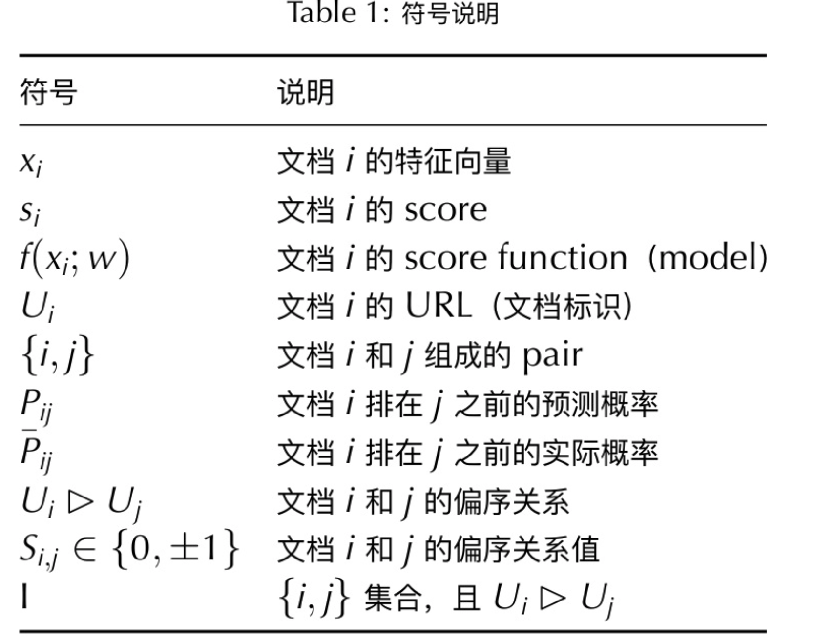
(Table from [9])
After reading the first three chapters of [7], you probably reach the plot:
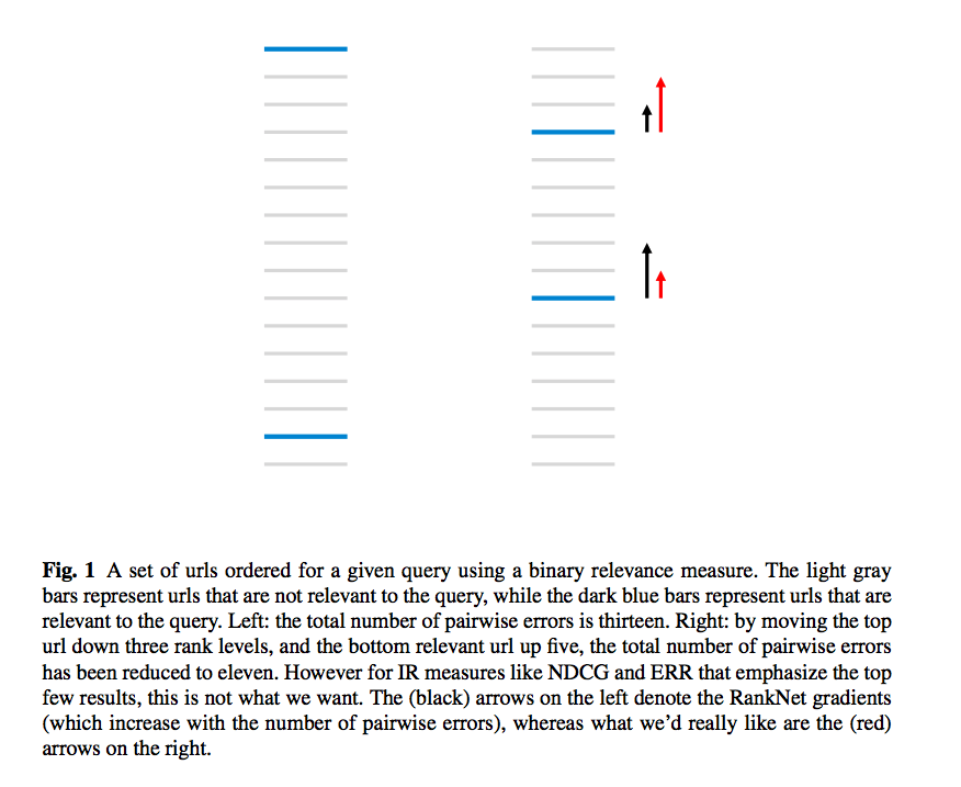
The plot illustrates the motivation for the invent of LambdaRank based on RankNet. In RankNet, the cost function is an easily defined, differentiable function:

If  ,
,  ; if ,
  . The intuition of this cost function is that the more consistent the relative order between
  and
and  is with
  , the smaller
  will be.
Since the scores and are from a score function of parameters  , the cost function is a function of too. Our goal is to adjust to minimize . Therefore, we arrive at the gradient of regarding (using just one parameter
  as example):
 , where
  . (This is from Eqn. 3 in [7].)
 is derived from a pair of URLs
  and
and  . For each document, we can aggregate to
  by taking into account of all its interaction with other documents:

Based on the derivation from Section 2.1 in [7], the update rule of score function parameter can be eventually expressed by :

can be seen as the force to drive high and low of from document . Here is how one can understand the effect of through a simple but wordy example. Suppose for a document which only has one pair  (). Assume in one particular update step, we have
  , i.e., an increase of will cause to increase if everything else is fixed. Therefore,
  assuming
  . According to the update rule
  , immediately we know that is going increase further to increase . Nevertheless, depending on whether
  or
or  , the scale of would be different. If , that is, the current calculated scores has a relative order consistent with the label, then
  . On the other hand, if
  , that is, the current calculated scores are inconsistent with the label,
  will become relatively large (
 1).
1).
3. LambdaMART
The problem of RankNet is that sometimes does not perfectly correlate to the force we want to drag the document to the ideal place. On the right of the example plot, the black arrows denote the blue documents are assigned. However, if we want to use metrics that emphasize on the top few results (e.g., NDCG/ERR) we want to correlate with the red arrows. Unfortunately, many metrics like NDCG and ERR are not easy to come up with a well-formed cost function . Recall the cost function of RankNet: as long as and are consistent with , will be low regardless the absolution positions that and appear. The fortunate part is that we do not need to know when we train the model: all we need to know is and we can design our own for those not well-formed cost functions. Thus, the core idea of LambdaRank is to define by:

where  is the change after swapping and of any measure you apply. This swap takes place in the sorted list of all documents according to their current calculated scores, and all documents’ positions are kept fixed except the two documents being swapped.
Now, if the model we are training contains parameters that form differential score functions then we can easily apply the update rule on those parameters like we talked about in <2. RankNet>: 
However, if we are going to train MART, then we need to train it according to its iterative process, which only requires knowing . This finally arrives at the LambdaMART algorithm:
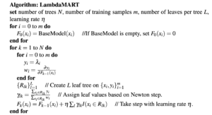
Note that in LambdaMART we usually define in the way that fitting it is equivalent to maximizing some utility function . Therefore, the Newton step to calculate  is actually doing gradient ascent. Recall that in <1. MART> section the objective that each MART tree optimizes for is:

In the LambdaMART algorithm,  corresponds to
  and
and  corresponds to
  .
.
Reference
[1] http://www.cnblogs.com/wowarsenal/p/3900359.html
[2] https://www.quora.com/search?q=lambdamart
[3] https://liam0205.me/2016/07/10/a-not-so-simple-introduction-to-lambdamart/
[5] https://www.slideshare.net/Julian.Qian/learning-to-rank-an-introduction-to-lambdamart
[6] https://en.wikipedia.org/wiki/Newton%27s_method
[8] https://www.youtube.com/watch?v=IXZKgIsZRm0
[9] https://www.slideshare.net/Julian.Qian/learning-to-rank-an-introduction-to-lambdamart
[10] http://xgboost.readthedocs.io/en/latest/model.html
[11] https://stats.stackexchange.com/questions/157870/scikit-binomial-deviance-loss-function
[13] http://dasonmo.cn/2019/02/08/from-ranknet-to-lambda-mart/
Update 2020/02/22:
This reference contains an example of computing using NDCG metric:
[14] http://dasonmo.cn/2019/02/08/from-ranknet-to-lambda-mart/