More details in DPO

In this post, we dig into more details of Direct Preference Optimization [1], a popular method used in RLHF.

First, we start from the normal RLHF objective that is typically used in PPO literature, which is equation 3 in the DPO paper [1].

\max_{\pi_\theta} \mathbb{E}_{x \sim \mathcal{D}, y\sim \pi_\theta(y|x)}[r_\phi(x,y)] - \beta \mathbb{D}_{KL}[\pi_\theta(y|x) || \pi_{ref}(y|x)],
which states that we want to maximize the reward model score r_\phi(x,y) but also, in balance, to minimize the KL-divergence from a reference policy \pi_{ref}(y|x)

The equation above can be rewritten by incorporating the KL-divergence term into the reward function. Because \mathbb{D}_{KL}[\pi_\theta(y|x) || \pi_{ref}(y|x)]=\sum_y \pi_\theta(y|x) \log\frac{\pi_\theta(y|x)}{\pi_{ref}(y|x)} =\mathbb{E}_{y\sim \pi_\theta(y|x)}[\log\frac{\pi_\theta(y|x)}{\pi_{ref}(y|x)}], we have

\max_{\pi_\theta} \mathbb{E}_{x \sim \mathcal{D}, y\sim \pi_\theta(y|x)}\left[r_\phi(x,y) - \beta (\log \pi_\theta(y|x) - \log \pi_{ref}(y|x)) \right] \newline = \mathbb{E}_{x \sim \mathcal{D}, y\sim \pi_\theta(y|x)}\left[r_\phi(x,y) + \beta \log \pi_{ref}(y|x) - \beta \log \pi_\theta(y|x) \right] \newline \text{because }-\log \pi_\theta(y|x) \text{ is an unbiased estimator of entropy } H(\pi_\theta)=-\sum_y \pi_\theta(y|x) \log \pi_\theta(y|x),  \newline \text{we can transform to equation 2 in [3]} \newline= \mathbb{E}_{x \sim \mathcal{D}, y\sim \pi_\theta(y|x)}\left[r_\phi(x,y) + \beta \log \pi_{ref}(y|x) + \beta H(\pi_\theta)\right] 


Now there are two perspectives for how to solve the maximization problem above. The first solution is based on the DPO paper’s Appendix A.1:


Reference

  1. Direct Preference Optimization: Your Language Model is Secretly a Reward Model: https://arxiv.org/abs/2305.18290
  2. Reinfocement Learning in LLMs: https://czxttkl.com/2024/01/23/reinfocement-learning-in-llms/
  3. From r to Q∗: Your Language Model is Secretly a Q-Function: https://arxiv.org/abs/2404.12358
  4. Controlled decoding from language models: https://arxiv.org/abs/2310.17022

Minimal examples of HuggingFace LLM training

I’m sharing a minimal example of training an LLM model using HuggingFace’s libraries trl/transformers/evaluate/datasets/etc. The example is mainly borrowed from https://wandb.ai/capecape/alpaca_ft/reports/How-to-Fine-tune-an-LLM-Part-3-The-HuggingFace-Trainer–Vmlldzo1OTEyNjMy and its github repo https://github.com/tcapelle/llm_recipes/blob/main/scripts/train_hf.py.

Here is the full file:

import wandb
from datasets import load_dataset

# if you can't find libwebp library, use brew update && brew install webp
import evaluate
import numpy as np
import torch
from transformers import TrainingArguments
from trl import SFTTrainer
from transformers import (
    AutoModelForCausalLM, AutoTokenizer, AutoConfig,
    LlamaConfig, LlamaModel,
)
from transformers import GenerationConfig
from transformers.integrations import WandbCallback
from tqdm import tqdm


def token_accuracy(eval_preds):
    token_acc_module = evaluate.load("accuracy")
    logits, labels = eval_preds
    # shape: batch_size x max_sequence_length
    predictions = np.argmax(logits, axis=-1)
    # accuracy only accepts 1d array. So if the batch contains > 1 datapoints,
    # the accuracy is based on flattened arrays
    # https://huggingface.co/spaces/evaluate-metric/accuracy
    return token_acc_module.compute(
        predictions=predictions.flatten().astype(np.int32),
        references=labels.flatten().astype(np.int32),
    )


def prompt_no_input(row):
    return ("Below is an instruction that describes a task. "
            "Write a response that appropriately completes the request.\n\n"
            "### Instruction:\n{instruction}\n\n### Response:\n{"
            "output}").format_map(
        row
    )


def prompt_input(row):
    return (
        "Below is an instruction that describes a task, paired with an input "
        "that provides further context. "
        "Write a response that appropriately completes the request.\n\n"
        "### Instruction:\n{instruction}\n\n### Input:\n{input}\n\n### "
        "Response:\n{output}").format_map(
        row
    )


def create_alpaca_prompt(row):
    return prompt_no_input(row) if row["input"] == "" else prompt_input(row)


class LLMSampleCB(WandbCallback):
    def __init__(
            self, trainer, test_dataset, num_samples=10, max_new_tokens=256,
            log_model="checkpoint"
    ):
        super().__init__()
        self._log_model = log_model

        def create_prompt_no_anwer(row):
            row["output"] = ""
            return {"text": create_alpaca_prompt(row)}

        self.sample_dataset = test_dataset.select(range(num_samples)).map(
            create_prompt_no_anwer
        )
        self.model, self.tokenizer = trainer.model, trainer.tokenizer
        self.gen_config = GenerationConfig.from_pretrained(
            trainer.model.name_or_path,
            max_new_tokens=max_new_tokens
        )

    def generate(self, prompt):
        tokenized_prompt = self.tokenizer(prompt, return_tensors='pt')[
            'input_ids']
        with torch.inference_mode():
            output = self.model.generate(
                inputs=tokenized_prompt, generation_config=self.gen_config
            )
        return self.tokenizer.decode(
            output[0][len(tokenized_prompt[0]):], skip_special_tokens=True
        )

    def samples_table(self, examples):
        records_table = wandb.Table(
            columns=["prompt", "generation"] + list(
                self.gen_config.to_dict().keys()
            )
        )
        for example in tqdm(examples):
            prompt = example["text"]
            generation = self.generate(prompt=prompt)
            records_table.add_data(
                prompt, generation, *list(self.gen_config.to_dict().values())
            )
        return records_table

    def on_evaluate(self, args, state, control, **kwargs):
        super().on_evaluate(args, state, control, **kwargs)
        records_table = self.samples_table(self.sample_dataset)
        self._wandb.log({"sample_predictions": records_table})
        print("log once")


def param_count(m):
    params = sum([p.numel() for p in m.parameters()]) / 1_000_000
    trainable_params = sum(
        [p.numel() for p in m.parameters() if p.requires_grad]
    ) / 1_000_000
    print(f"Total params: {params:.2f}M, Trainable: {trainable_params:.2f}M")
    return params, trainable_params


def trl_train():
    wandb.login(key='replace_with_your_own')

    lr = 2e-5
    batch_size = 8
    max_steps = 4
    # evaluate every eval_steps. so if we set max_steps = 4 and
    # eval_steps = 2, we will evaluate twice during training
    eval_steps = 2
    num_eval_data = 5
    num_wandb_cb_eval_data = 7
    wandb_cb_max_new_tokens = 256
    num_train_epochs = 1
    max_seq_length = 1024
    gradient_accumulation_steps = 1
    gradient_checkpointing = False
    output_dir = "./output/"

    run = wandb.init(
        project="second_project",
        config={
            "lr": lr,
            "batch_size": batch_size,
            "max_steps": max_steps,
            "eval_steps": eval_steps,
            "num_eval_data": num_eval_data,
            "num_wandb_cb_eval_data": num_wandb_cb_eval_data,
        },
    )

    alpaca_ds = load_dataset("winglian/alpaca-gpt4-split")

    train_dataset = alpaca_ds["train"]
    eval_dataset = alpaca_ds["test"]

    model_id = 'meta-llama/Llama-2-7b-hf'
    # try different ways to initialize a llama model
    # method 1: construct LLamaModel from LlamaConfig
    # https://huggingface.co/docs/transformers/v4.37.2/en/model_doc
    # /llama2#transformers.LlamaConfig
    # configuration = LlamaConfig(
    #     num_hidden_layers=2,
    #     hidden_size=32,
    #     intermediate_size=2,
    #     num_attention_heads=1,
    #     num_key_value_heads=1,
    # )
    # model = LlamaModel(configuration)
    # param_count(model)

    # method 2 & 3 need to wait for token approval
    # https://huggingface.co/meta-llama/Llama-2-7b-hf
    # method 2: load config first, tune down model size, then initialize the actual LLM
    # https://discuss.huggingface.co/t/can-i-pretrain-llama-from
    # -scratch/37821/8
    config = AutoConfig.from_pretrained(model_id)
    config.num_hidden_layers = 1
    config.hidden_size = 2
    config.intermediate_size = 2
    config.num_attention_heads = 1
    config.num_key_value_heads = 1
    model = AutoModelForCausalLM.from_config(config)
    param_count(model)

    # method 3: directly load pretrained llama model, which may encounter OOM
    # on a consumer cpu machine
    # model = AutoModelForCausalLM.from_pretrained(
    #     model_id,
    #     device_map="auto",
    #     trust_remote_code=True,
    #     low_cpu_mem_usage=True,
    #     torch_dtype=torch.bfloat16,
    #     load_in_8bit=True,
    # )

    training_args = TrainingArguments(
        output_dir=output_dir,
        use_cpu=True,
        report_to="wandb",
        per_device_train_batch_size=batch_size,
        bf16=True,
        learning_rate=lr,
        lr_scheduler_type="cosine",
        warmup_ratio=0.1,
        max_steps=max_steps,
        eval_steps=eval_steps,
        num_train_epochs=num_train_epochs,
        gradient_accumulation_steps=gradient_accumulation_steps,
        gradient_checkpointing=gradient_checkpointing,
        gradient_checkpointing_kwargs={"use_reentrant": False},
        evaluation_strategy="steps",
        # logging strategies
        logging_strategy="steps",
        logging_steps=1,
        save_strategy="no",
    )
    tokenizer = AutoTokenizer.from_pretrained(model_id)
    tokenizer.pad_token = tokenizer.eos_token

    trainer = SFTTrainer(
        model,
        tokenizer=tokenizer,
        args=training_args,
        train_dataset=train_dataset,
        eval_dataset=eval_dataset.select(list(range(num_eval_data))),
        # this tells the trainer to pack sequences of `max_seq_length`
        # see illustration in https://wandb.ai/capecape/alpaca_ft/reports/How
        # -to-Fine-tune-an-LLM-Part-3-The-HuggingFace-Trainer--Vmlldzo1OTEyNjMy
        packing=True,
        max_seq_length=max_seq_length,
        formatting_func=create_alpaca_prompt,
        compute_metrics=token_accuracy,  # only call at evaluation
    )
    wandb_callback = LLMSampleCB(
        trainer, eval_dataset,
        num_samples=num_wandb_cb_eval_data,
        max_new_tokens=wandb_cb_max_new_tokens,
    )
    trainer.add_callback(wandb_callback)
    trainer.train()
    wandb.finish()

    # other materials:
    # fine tune ppo vs dpo
    # trl stackllama tutorial:
    # https://huggingface.co/docs/trl/using_llama_models
    # trl readme: https://github.com/huggingface/trl/tree/main?tab=readme-ov
    # dpo - trl: https://huggingface.co/blog/dpo-trl


if __name__ == '__main__':
    trl_train()

Now let’s examine the code in more details:

First, we initialize a weights & bias project (wandb.init(...)), which is used for logging intermediate training/evaluation results. It is a very convenient tool for logging and visualization. 

Then, we use  load_dataset(...) , an api from HuggingFace’s dataset library, to load a specific data. HuggingFace hosts many awesome datasets at https://huggingface.co/datasets.

Next, we initialize an actual LLM. Since this is a minimal example, I created a tiny LLM by modifying its config to have very few hidden layers and hidden sizes.

Next, we initialize TrainingArguments. We may need to be familiar with several concepts in TrainingArguments, such as gradient accumulation

We then initialize a tokenizer, which is trivial by calling HuggingFace’s API AutoTokenizer.from_pretrained(...)

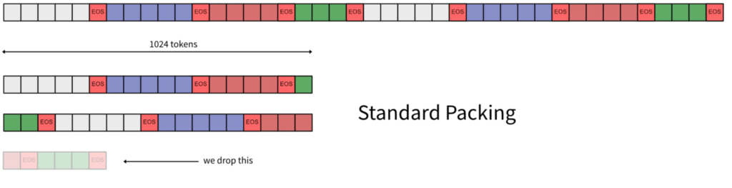
We then initialize SFTTrainer, the main class for training and evaluating the LLM. Setting packing=True means that we pack multiple individual sequences into a fixed-length sequence so that we can avoid much padding. Individual sequences are usually separated with an eos token.

We also initialize a callback, which is called only in the evaluation stage. The callback class needs to first remove output in the dataset for evaluation.


We now look at the results logged in wandb (example https://wandb.ai/czxttkl/third_project/runs/hinck0h5):

  1. Since we specify max_steps=4 and eval_steps=2, we have 2 evaluations. The evaluation loss curves verifie we indeed log 2 evaluation results.
  2. we have a table showing the results from the callback. We can verify that prompts indeed have outputs removed. We can also use runs.history.concat["sample_predictions"] instead of runs.summary["sample_predictions"] to check the evaluation results from all evaluation runs (exactly 2 runs) (see the reference in https://wandb.ai/morg/append-to-table/reports/Append-to-Table–Vmlldzo0MjY0MDIx)


Causal Inference 102

In my blog, I have covered several pieces of information about causal inference: 

  1. Causal Inference: we talked about (a) two-stage regression for estimating the causal effect between X and Y even when there is a confounder between them; (b) causal invariant prediction
  2. Tools needed to build an RL debugging tool: we talked about 3 main methods for causal relationship discovery – (a) noise model; (b) quantile regression with the idea of Kolmogorov complexity; (c) matching
  3. Causal Inference in Recommendation Systems: we talked about backdoor/frontdoor adjustment and causal relationship discovery in a sequence modeling setting

This time, I read a paper about learning causal relationship from pure observational data [1]. It has a very clear introduction of causal inference, which inspires me to write another introduction post of causal inference.

Let’s start from basic definitions. Structural causal models (SCM), structural equation models (SEM), or functional causal models (FCM) all refer to the same thing: a graph which indicates causal relationships between nodes and causal relationships are encoded by functions and noises. [1] uses the notation of FCM primarily. Here is an example of an FCM:

collider definition [5]: if a node has two edges pointing to it, it is called a collider. In the example above, x5 is a collider. X3, X4, and X5 form the so-called “v-structure”.

d-separation definition: d-separation is used to determine if a node set X is independent of a node set Y, given a node set Z. Specifically, if X and Y are d-connected, then X and Y are dependent given Z, denoted as X \not\!\perp\!\!\!\perp_G Y | Z; if X and Y are d-separated, then X and Y are independent given Z, denoted as  X \perp\!\!\!\perp_G Y | Z. If two nodes are not d-connected, then they are d-separated. There are several rules for determining whether two nodes are d-connected or d-separated [3]. An interesting (and often non-intuitive) example is that in a v-structure like (X3, X4, X5) above: X3 is d-connected (i.e., dependent) to X4 given X5 (i.e., the collider), even though X3 and X4 has no direct edge in between [4].

Identifiability definition: An observational distribution of all variables could be resulted by different FCMs. Thus, we are not guaranteed to infer the correct causal relationship from observational data. That’s why FCM is a richer structure than pure observational data and using pure probabilistic distributions are not enough to do causal inference! Proposition 4.1 (non-uniqueness of graph structures) in [6] says that there will always be some graph structure to explain an observational data of two variables thus we can never determine the correct causal relationship without additional assumption. If, with correct assumptions, we can identify the ground truth FCM from observational data, we call the FCM is identifiable.

Faithfulness definition: We are given observational data and a hypothesized FCM. Running conditional independence tests on the observational distribution will give us all conditional independence relationships. If all the identified conditional independence relationships from the data are also entailed by the FCM, then the observational distribution is faithful to the FCM. Here is an example [7] that an observational distribution is unfaithful to an FCM:

  1. In the FCM, we can see that A and D are d-connected, meaning A and D are dependent (given an empty set Z).
  2. If A, B, C, and D have the linear relationships indicated as on the right, then D=(\alpha\beta + \gamma\delta)A. When \alpha\beta =- \gamma\delta, the conditional independence test will return us \perp\!\!\!\perp. Therefore, the identified conditional independence relationship from the data is not entailed by the FCM.

In practice, inferring FCMs from observational data are based on the Causal Sufficiency Assumption (CSA), Causal Markov Assumption (CMA), and Causal Faithfulness Assumption (CFA) (more details in [1]). Based on these assumptions, inferring FCMs from observational data limits the space of plausible FCMs and involves the following steps:

  1. Determine all possible causal relationships using conditional independent tests and derive the Completed Partially Directed Acyclic Graph (CPDAG)
  2. For undeterminable causal relationships, use constraint-based methods, score-based methods, or hybrid methods to get the best hypothesis

Recall that based on non-uniqueness of graph structures, there will always be some graph structure to explain an observational data of two variables thus we can never determine the correct causal relationship without additional assumption. Now let’s look at what additional assumption we could have to facilitate causal discovery in real world:

  1. LinGAM assumes a linear structure FCM with all variables are continuous:
    X_i = \sum\limits_k \alpha_k P_a^k(X_i)+E_i, \;\; i \in [1, N]
    The LinGAM paper proves that when all probability distributions of source nodes in the causal graph are non-Gaussian, FCM is fully identifiable. 
  2. The additive noise model (ANM) assumes that we can learn the true causal direction between X and Y when:
    1. Y=f(X)+E
    2. f(\cdot) is not a linear model with Gaussian input and Gaussian noise
    3. Only two variables are involved in the FCM (hence ANM is a bivariate method)
  3. The causal additive model (CAM) is the counterpart of ANM when there are more than 2 variables. Its assumption is similar to ANM that f(\cdot)  cannot be a linear model with Gaussian input and Gaussian noise for the FCM to be identifiable. (I am not totally sure about CAM’s assumption. We may need to verify more carefully.)


Up to this point, we have finished the causal inference 102 introduction. The proposed method itself in [1] is interesting and useful to me because I need to conduct causal relationship discovery on observational data very often. And its neural network-based method seems general to handle practical data. There are many other causal relationship discovery methods. You can find more in an open source toolbox: [2]


References

[1] Learning Functional Causal Models with Generative Neural Networks: https://arxiv.org/abs/1709.05321

[2] https://fentechsolutions.github.io/CausalDiscoveryToolbox/html/causality.html

[3] https://yuyangyy.medium.com/understand-d-separation-471f9aada503

[4] https://stats.stackexchange.com/a/399010/80635

[5] https://en.wikipedia.org/wiki/Collider_(statistics)

[6] Elements of Causal Inference: https://library.oapen.org/bitstream/handle/20.500.12657/26040/11283.pdf?sequence=1&isAllowed=y

[7] https://www.youtube.com/watch?v=1_b7jgupoAE


Reinfocement Learning in LLMs

In this post, we overview Reinforcement Learning techniques used in LLMs and alternative techniques that are often compared with RL techniques.

PPO

The PPO-based approach is the most famous RL approach. Detailed derivation of PPO and implementation tricks are introduced thoroughly in [2]. Especially, we want to call out their recommended implementation tricks:

SLiC-HF

SLiC-HF [1] is a technique often compared with RLHF. Its idea is straightforward: for a human preference dataset, (x, y^+, y^-,), we penalize the unfavored output y^- with a hinge loss:

L(\theta)=max(0, \beta - log P_\theta(y^+|x) + log P_\theta(y^-|x))

SLiC-HF eliminates the need to train a reward model so it greatly simplifies the alignment process compared to PPO-based approaches.


DPO

In the same vein to eliminate the need to train a separate reward model, Direct Preference Optimization (DPO) proposes that we can directly fine-tune a LLM policy \pi_\theta(y|x) (the initial policy is denoted as \pi_{ref}(y|x)) with the loss:

There are many ways to interpret this loss. One intuitive one is that we will bump the likelihood of generating winning responses y_w and lower the likelihood of losing responses y_l under a Bradley-Terry model.


References

  1. SLiC-HF: Sequence Likelihood Calibration with Human Feedback: https://arxiv.org/abs/2305.10425
  2. Secrets of RLHF in Large Language Models Part I: PPO: https://arxiv.org/abs/2307.04964
  3. Direct Preference Optimization: Your Language Model is Secretly a Reward Model: https://arxiv.org/abs/2305.18290


Llama code anatomy

This is the first time I have read llama2 code. Many things are still similar to the original transformer code, but there are also some new things. I am documenting some findings.

Where is Llama2 Code?

Modeling (training) code is hosted here: https://github.com/facebookresearch/llama/blob/main/llama/model.py

Inference code is hosted here: https://github.com/facebookresearch/llama/blob/main/llama/generation.py

Annotations

There are two online annotations for llama2 code which I think are useful:

  1. [Ref1] Deciphering the LLAMA2 Code: Unraveling the Secrets of a Language AI Marvel: https://www.linkedin.com/pulse/deciphering-llama2-code-unraveling-secrets-language-ai-ayoub-kirouane/
  2. [Ref2] The Annotated LLaMA: https://medium.com/@nishantbhansali80/the-annotated-llama-fa183943b34b

While the two annotations are useful, I still need some external references for parts I don’t understand:

  1. precompute_freqs_cis is a function for computing rotary embeddings. Ref2 has a better explanation than Ref1.

  2. K/V cache (self.cache_k and self.cache_v in Attention class) is only meaningfully useful in inference (next token prediction). First, we need to build a mental model how inference works. Suppose we have a batch of prompts to start the inference (of the same length for simplicity). The transformer model will consume the batch of prompts and generate the first tokens. Then, each next token will be generated by consuming the prompts + previously generated tokens. If we don’t have K/V cache, you can foresee that K/V will be repeatedly computed for previously generated sequences for each next token. 
    K/V cache eliminates the need to recompute K/V after predicting every next token. With K/V cache, self.cache_k and self.cache_v will store the current batch’s K/V and K/V of the full previously generated sequences will be fetched from self.cache_k and self.cache_v (https://github.com/facebookresearch/llama/blob/main/llama/model.py#L276-L283):
    To help understand more, you can see that the forward function of Attention accepts start_pos as an argument (https://github.com/facebookresearch/llama/blob/main/llama/model.py#L265). After the first batch which contains prompts, each following batch will contain single tokens that are generated from the last batch. Therefore, start_pos will be +1 incremental and every following batch’s seq_len will become 1. One can reference llama2 inference code: https://github.com/facebookresearch/llama/blob/main/llama/generation.py#L162-L212 for how a model really gets called in the inference time.
    A side note is that K/V cache reduces FLOPs but does not reduce overall decoding time complexity. Here is a table (similar to this post’s table) showing the FLOPs of each sub-step when predicting each new token:
      w/o K/V cache, x needs to have shape (batch_size * seq_len * hidden_dim) with K/V cache, x has shape (batch_size * 1 * hidden_dim)
    Convert x to K/V by xW_K, xW_V O(batch_size * seq_len * hidden_dim * hidden_dim)

    O(batch_size * 1 * hidden_dim * hidden_dim)

    K/V cache only saves this part’s FLOP

    Convert x[:, -1] to q by x[:, -1]W_Q O(batch_size * hidden_dim * hidden_dim) O(batch_size * hidden_dim * hidden_dim)
    p = softmax (qK^T) / sqrt(d) O(batch_size * seq_len * hidden_dim * hidden_dim)

    O(batch_size * seq_len * hidden_dim * hidden_dim)

    Overall time complexity is still dominated by softmax

    a = pV O(batch_size * seq_len * hidden_dim) O(batch_size * seq_len * hidden_dim)
    Convert a to output aW_O O(batch_size * hidden_dim * hidden_dim) O(batch_size * hidden_dim * hidden_dim)
     
  3. K/V/O linear transformation (https://github.com/facebookresearch/llama/blob/main/llama/model.py#L221-L234) is done using TensorParallelism (ColumnParallelLinear or RowParallelLinear), which is introduced in https://arxiv.org/pdf/1909.08053.pdf and explained in https://awsdocs-neuron.readthedocs-hosted.com/en/latest/libraries/neuronx-distributed/tensor_parallelism_overview.html and https://www.cnblogs.com/rossiXYZ/p/15871062.html#0x04-rowparallellinear. At a high level, TensorParallelism chunks original large matrices into smaller ones, put them on different GPUs, and collect results only when needed, so as to speed up matrix operation.

Improve reasoning for LLMs

LLMs have become the hottest topic in 2023, when I did not have much time to cover related topics. Let’s deep dive into this topic in the beginning of 2024.

Prompts

Using few-shots prompts to hint LLMs how to solve problems is the simplest form to improve reasoning for LLMs. When you first come across LLMs, you will be surprised that prompting can be a methodology to improve reasoning, even though it seems only like a game of language manipulation. 

Here are prompting techniques I have encountered:

  1. Chain of Thought [2]: for every question to an LLM, we augment the question with a few exemplars (termed “few-shot learning by prompting”). Instead of directly showing answers in the exemplars, the exemplars contain detailed reasoning steps one by one, hence encourages the LLM to output step-by-step answers to the actual question.
  2. Resprompt [1]: more like a graph version of the linear version of chain of thought. The motivation is that “later stages often depend on the results of several steps earlier, not just the results of the immediately preceding step”. 
  3. Step-back prompting [3]. It also uses “few-shot learning by prompting” to improve LLMs’ reasoning. Each exemplar consists of two steps: ask a generic question about a high-level principle or concept behind the original question; then ground the reasoning on step 1’s answer. The two steps are also called “abstraction-and-reasoning”, which demonstrates that it is hard for LLMs to directly address very specific questions but relatively easier if deriving a high level concept first.
  4. React prompting [5]. This type of prompting is suited when the LLM can perform actions in multiple rounds (e.g., calling a search engine) to acquire external knowledge. React prompting is also a few shot learning technique, which contains a few exemplars of interleaving actions and reasoning traces. The picture below is an exemplar in a few-shot prompt. There are more examples in the paper’s Appendix C [5].
  5. Automatic prompt optimization [8]. The works introduces a search-based optimization process similar to Monte-Carlo Tree Search to iteratively find the best prompt which can get the highest score (based on a given metric function on a given dataset).   

Improve Reward Model

OpenAI shows a way [4] to improve reward models which can consequently improve the LLM model’s reasoning. Typically an outcome-supervised reward model is trained to output a scalar based on the whole input and output sequence. Rather, [4] collects a step-by-step solution dataset which is generated by a LLM on math problems and annotated per-step correctedness by human labelers. Then, [4] trains a “process-supervised reward model” to predict the correctness of each step. If we take the product of each step’s correctness probability, we get the final answer’s correctness probability. [4] evaluates the process-supervised reward model and the typical outcome-supervised reward model: by sampling N step-by-step solutions from a LLM and picking the best one with the highest reward, the process-supervised reward model solves more problems on average than the outcome-supervised reward model.

The West-of-N paper [12] introduces an interesting semi-supervised learning idea to augment human preference data with synthetic preference data to boost reward model performance. When we perform rejection sampling, we get sampled responses and their reward scores (with an incumbent reward model). We can pick the two responses with the highest and lowest score to form synthetic preference pairs as an additional dataset to retrain the reward model. The results show that the reward model improves due to this semi-supervised learning paradigm, “with an effect comparable to the addition of a similar quantity of human preference data”.


Introduce additional loop

Self-Training [10] adopts two stages to SFT LLMs. The first stage is called Grow, where a batch of data is sampled using the current LLM and scored by a RM. The second stage is called Improve, where the LLM is trained with the SFT objective. We can perform multiple Grow and Improve iterations to improve the LLM’s capability. RAFT [11] is a special case of Self-Training in which there is only one Improve iteration after Grow stage.

Self-consistency [7] is an example to introduce an additional loop to sample multiple solutions from Chain-of-Thought prompts. The sampled solutions are then marginalized (e.g., majority vote) to get the most convincing solution. A common and simple baseline to compare self-consistency with is to sample the same number of solutions from an LLM and get the best one with the highest decoding probability. Self-consistency beats this baseline by a significant margin, indicating that decoding probabilities are not a good indicator of solution quality [9].  

Reflexion [6] is an more complex example to introduce a loop to improve LLMs over time. An LLM-based actor outputs answers given prompts, an evaluator evaluates the actor’s answer (evaluator can be a verification function for logic tasks or an LLM for NLP tasks), and an LLM-based self-reflection component evaluates how the actor’s answer leads to the evaluation result and then stores useful lessons in a long-term memory for the actor’s future usage.


References

[1] Resprompt: Residual Connection Prompting Advances Multi-Step Reasoning in Large Language Models: https://arxiv.org/abs/2310.04743

[2] Chain-of-Thought Prompting Elicits Reasoning in Large Language Models: https://arxiv.org/abs/2201.11903

[3] Take a Step Back: Evoking Reasoning via Abstraction in Large Language Models: https://arxiv.org/abs/2310.06117

[4] Let’s Verify Step by Step: https://arxiv.org/abs/2305.20050

[5] ReAct: Synergizing Reasoning and Acting in Language Models: https://arxiv.org/abs/2210.03629

[6] Reflexion: Language Agents with Verbal Reinforcement Learning: https://arxiv.org/abs/2303.11366

[7] Self-Consistency Improves Chain of Thought Reasoning in Language Models: https://arxiv.org/abs/2203.11171

[8] Automatic Prompt Optimization with “Gradient Descent” and Beam Search: https://arxiv.org/abs/2305.03495

[9] Calibrating Sequence likelihood Improves Conditional Language Generation: https://arxiv.org/abs/2210.00045

[10] Reinforced Self-Training (ReST) for Language Modeling: https://arxiv.org/abs/2308.08998

[11] RAFT: Reward rAnked FineTuning for Generative Foundation Model Alignment: https://arxiv.org/abs/2304.06767

[12] West-of-N: Synthetic Preference Generation for Improved Reward Modeling: https://arxiv.org/abs/2401.12086


Dollar cost average on TQQQ vs QQQ [Real Data]

(Please cross reference to my previous post for simulation-based results: https://czxttkl.com/2023/01/15/dollar-cost-average-on-tqqq-vs-qqq/)

In this post, we use real data (from 2021 april to 2024 jan) to show that even after a bear market (in 2022), DCA on TQQQ is still more profitable than QQQ. UPRO is also more profitable than SPY but the margin is not that significant. 

# https://stockcharts.com/h-sc/ui

import yfinance as yf


def my_stock_return(tick):
    stock = yf.Ticker(tick)
    stock_hist = stock.history(start="2021-04-01", end="2024-01-12")
 
    days = 0
    total_share = 0
    single_invest = 3000
    total_invest = 0
    total_invest_time = 0
    for idx, row in stock_hist.iterrows():
        if days % 10 == 0:
            single_share = single_invest / row['Open']
            total_share += single_share
            total_invest += single_invest
            total_invest_time += 1

        days += 1

    total_value = total_share * stock_hist.iloc[-1]["Close"]

    print(f"tick={tick}")
    print(f"days: {days}")
    print(f'last day close: {stock_hist.iloc[-1]["Close"]}')
    print(f"total_share: {total_share}")
    print(f'total_value = total_share * last day close: {total_value}')
    print(f"total_invest: {total_invest}, total_invest_time: {total_invest_time}")
    print(f"total gain: {(total_value / total_invest - 1) * 100}%")


my_stock_return("TQQQ")
print("\n")
my_stock_return("QLD")
print("\n")
my_stock_return("QQQ")
print("\n")
my_stock_return("UPRO")
print("\n")
my_stock_return("SPUU")
print("\n")
my_stock_return("SPY")
print("\n")

Here is the result:

tick=TQQQ
days: 700
last day close: 50.279998779296875
total_share: 5908.547006195283
total_value = total_share * last day close: 297081.736258917
total_invest: 210000, total_invest_time: 70
total gain: 41.467493456627146%


tick=QLD
days: 700
last day close: 75.68000030517578
total_share: 3737.0006961799377
total_value = total_share * last day close: 282816.2138273398
total_invest: 210000, total_invest_time: 70
total gain: 34.674387536828476%


tick=QQQ
days: 700
last day close: 409.3500061035156
total_share: 636.3171528636028
total_value = total_share * last day close: 260476.4304084875
total_invest: 210000, total_invest_time: 70
total gain: 24.03639543261309%


tick=UPRO
days: 700
last day close: 54.790000915527344
total_share: 4596.7168995484735
total_value = total_share * last day close: 251854.12313468088
total_invest: 210000, total_invest_time: 70
total gain: 19.930534826038503%


tick=SPUU
days: 700
last day close: 103.43000030517578
total_share: 2430.3500485571817
total_value = total_share * last day close: 251371.1062639533
total_invest: 210000, total_invest_time: 70
total gain: 19.70052679235872%


tick=SPY
days: 700
last day close: 476.3500061035156
total_share: 508.7714829247962
total_value = total_share * last day close: 242353.29899652136
total_invest: 210000, total_invest_time: 70
total gain: 15.40633285548636%

Result analysis:

  1. DCA on TQQQ is more profitable than QYD (2x) and QQQ (1x). 
  2. UPRO is as profitable as SPUU (2x) while it took more risk during the bear market
  3. UPRO is only 4% more profitable than SPY. 
 

Diffusion models

Diffusion models are popular these days. This blog [1] summarizes the comparison between diffusion models with other generative models:

Before we go into the technical details, I want to use my own words to summarize my understanding in diffusion models. Diffusion models have two subprocesses: forward process and backward process. The forward process is non-learnable and the backward process is learnable. For every training samples (e.g., images) \mathbf{x}_0, the forward process adds a Gaussian noise \boldsymbol{\epsilon}_t in T steps until \mathbf{x}_T is (or approximately close to) an isotropic Gaussian. The backward process tries to recover \mathbf{x}_0 in T steps, starting from an isotropic Gaussian \mathbf{x}_T. Each backward step samples \mathbf{x}_{t-1} from \mathbf{x}_t with the probability p_\theta(\mathbf{x}_{t-1} | \mathbf{x}_{t}) = \mathcal{N}(\mathbf{x}_{t-1}| \boldsymbol{\mu}_\theta(\mathbf{x}_t, t), \Sigma_\theta(\mathbf{x}_t, t)). The eventual goal is that, given a training sample, we want p_\theta(\mathbf{x}_0) to be as high as possible, where p_\theta(\mathbf{x}_0)=p_\theta(\mathbf{x}_{T:0})=p(\mathbf{x}_T)\prod\limits_{t=T}^1 p_\theta(\mathbf{x}_{t-1} | \mathbf{x}_{t}). It turns out that maximizing p_\theta(\mathbf{x}_0) will be equivalent to optimizing an ELBO objective function, which is equivalent to make p_\theta(\mathbf{x}_{t-1} | \mathbf{x}_{t}) be as close as possible to the distribution q(\mathbf{x}_{t-1} | \mathbf{x}_{t}, \boldsymbol{\epsilon}_t). Because in the forward process we have recorded \mathbf{x}_t and \boldsymbol{\epsilon}_t for all t=1,\cdots, T, q(\mathbf{x}_{t-1} | \mathbf{x}_{t}, \boldsymbol{\epsilon}_t) can be written in a closed form. Therefore, we can use a loss function (i.e., KL divergence between two Gaussians) to train \theta by fitting p_\theta(\mathbf{x}_{t-1} | \mathbf{x}_{t}) against q(\mathbf{x}_{t-1} | \mathbf{x}_{t}, \boldsymbol{\epsilon}_t).      


More technical details

We start from the objective, that the data likelihood x_0 under a diffusion model \theta, is maximized: maximize \; \log p_\theta(x_0).  Similar to stochastic variational inference, we can derive a lower bound and maximize the lower bound instead:

(1)   \begin{equation*} \begin{split} & maximize \;\; \log p_\theta(x_0) \\  & \geq \log p_\theta(x_0) - \underbrace{D_{KL}\left( q\left( \mathbf{x}_{1:T} | \mathbf{x}_0 \right) || p_\theta\left( \mathbf{x}_{1:T} | \mathbf{x}_0 \right) \right)}_\text{KL divergence is non-negative} \\  &=\log p_\theta(x_0) - \mathbb{E}_{x_{1:T} \sim q(x_{1:T}|x_0) } \left[ \log \underbrace{\frac{q\left(\mathbf{x}_{1:T}|\mathbf{x}_0 \right)}{p_\theta\left( \mathbf{x}_{0:T}\right) / p_\theta \left( \mathbf{x}_0\right)}}_\text{Eqvlt. to $p_\theta\left( \mathbf{x}_{1:T} | \mathbf{x}_0 \right)$} \right] \\ &=\log p_\theta(x_0) - \mathbb{E}_{x_{1:T} \sim q(x_{1:T}|x_0) } \left[ \log \frac{q\left( \mathbf{x}_{1:T} | \mathbf{x}_0 \right)}{p_\theta \left( \mathbf{x}_{0:T}\right) } + \log p_\theta\left(\mathbf{x}_0 \right) \right] \\ &=- \mathbb{E}_{x_{1:T} \sim q(x_{1:T}|x_0) } \left[ \log \frac{q\left(\mathbf{x}_{1:T} | \mathbf{x}_0\right) }{p_\theta\left( \mathbf{x}_{0:T}\right)} \right] \\ &=-\mathbb{E}_{q}\biggl[ \\ &\quad \underbrace{D_{KL}\left( q( \mathbf{x}_T | \mathbf{x}_0) || p_\theta(\mathbf{x}_T) \right)}_\text{$L_T$} \\ &\quad + \sum\limits_{t=2}^T \underbrace{D_{KL}\left( q(\mathbf{x}_{t-1} | \mathbf{x}_t, \mathbf{x}_0) || p_\theta(\mathbf{x}_{t-1}|\mathbf{x}_t) \right)}_\text{$L_{t-1}$} \\ &\quad \underbrace{- \log p_\theta(\mathbf{x}_0 | \mathbf{x}_1)}_\text{$L_{0}$} \\ &\biggr] \end{split} \end{equation*}


We now focus on L_{t-1} for t=2, \cdots, T because L_T is non-learnable and L_0 is trivially handled. With some mathematical computation, we have 

(2)   \begin{equation*} q(\mathbf{x}_{t-1} | \mathbf{x}_t, \mathbf{x}_0) = \mathcal{N}(\mathbf{x}_{t-1}; \tilde{\boldsymbol{\mu}}(\mathbf{x}_t, \mathbf{x}_0), \tilde{\beta}_t \mathbf{I}) \end{equation*}

and

(3)   \begin{equation*} \begin{split} \tilde{\boldsymbol{\mu}}_t(\mathbf{x}_t, \mathbf{x}_0) &=\frac{\sqrt{\alpha_t}(1-\bar{\alpha}_{t-1})}{1-\bar{\alpha}_t}\mathbf{x}_t + \frac{\sqrt{\bar{\alpha}_{t-1}} \beta_t}{1-\bar{\alpha}_t} \mathbf{x}_0 \\ &= \frac{1}{\sqrt{\alpha_t}}\left( \mathbf{x}_t - \frac{1-\alpha_t}{\sqrt{1-\bar{\alpha}}_t } \epsilon_t\right),  \end{split} \end{equation*}

where \beta_t, \tilde{\beta}_t, and \bar{\alpha}_t are terms involving noise scheduling steps \alpha_t.


Now, the other part of L_{t-1} is p_\theta(\mathbf{x}_{t-1}|\mathbf{x}_t), which can be parameterized as

(4)   \begin{equation*} \begin{split} &p_\theta(\mathbf{x}_{t-1}|\mathbf{x}_t) \\ &= \mathcal{N}(\mathbf{x}_{t-1}; \boldsymbol{\mu}_\theta(\mathbf{x}_t, t), \boldsymbol{\Sigma}_\theta(\mathbf{x}_t, t) ) \\ &= \mathcal{N}(\mathbf{x}_{t-1}; \frac{1}{\sqrt{\alpha_t}} \Big( \mathbf{x}_t - \underbrace{\frac{1 - \alpha_t}{\sqrt{1 - \bar{\alpha}_t}} \boldsymbol{\epsilon}_\theta(\mathbf{x}_t, t)}_\text{predict $\epsilon_t$ from $\mathbf{x}_t$ and $t$} \Big), \boldsymbol{\Sigma}_\theta(\mathbf{x}_t, t)) \end{split} \end{equation*}

Because KL divergence betwen two Gaussians [5] can be represented as \mathrm{KL}[P\,||\,Q] = \frac{1}{2} \left[ (\mu_2 - \mu_1)^T \Sigma_2^{-1} (\mu_2 - \mu_1) + \mathrm{tr}(\Sigma_2^{-1} \Sigma_1) - \ln \frac{|\Sigma_1|}{|\Sigma_2|} - n \right], L_{t-1} (i.e., the KL divergence between p_\theta(\mathbf{x}_{t-1}|\mathbf{x}_t) and q(\mathbf{x}_{t-1} | \mathbf{x}_t, \mathbf{x}_0)) can be expressed analytically and fed into autograd frameworks for optimization.

Code Example

The exact code example I was reading is https://colab.research.google.com/github/JeongJiHeon/ScoreDiffusionModel/blob/main/DDPM/DDPM_example.ipynb, which is easy enough.

Our data is just two 2D Gaussian distributions. One distribution will be sampled more often (prob=0.8) than the other.     

And after 1000 training iterations, here is the inference process looks like: we have N data points which are pure Gaussian noises. p_\theta(\mathbf{x}_{t-1}|\mathbf{x}_t) are now learned such that sampling from it can recover the original data distribution (although I feel the two distributions are not 8-2 in quantities):


Mode collapse is real for generative models

I am very curious to see whether generative models like GAN and VAE can fit data of multi-modes. [1] has some overview over different generative models, mentioning that VAE has a clear probabilistic objective function and is more efficient.

[2] showed that diffusion models (score-based generative models) can better fit multimode distribution than VAE and GAN. [4] mentions that VAE does not have mode collapse as GAN but has a similar problem that the decoder may ignore the latent representation and generate things arbitrarily and InfoVAE [5] can mitigate it. [6] also suggested that beta-VAE and Adversarial VAE [7] achieve better performance than vanilla VAE. 

I did a hands-on toy experiment, where I generate 3-modes distributions and let vanilla VAE fit them. The result is not very satisfying given this is only a very simple toy problem. Therefore, it calls out that we may need more advanced VAE as described above.

First, when the three modes are well separated and well balanced (I generated 33% data as -10, 33% data as 0, and the other 33% data as 10):

However, when the three modes are -1, 0, and 1, generated data are not well separated:

When the three modes are -0.1, 0, and 0.1, generated data only concentrate on one mode (mode collapse!):

I also tried that the three modes have imbalanced data amount and VAE did not perform well either:


The toy experiment’s code can be found in `train_VAE_simple.py` in https://www.dropbox.com/sh/n8lbdzvrdvahme7/AADFgs_JLz8BhHzOaUCcJ1MZa?dl=0.

At last, I’d like to share that [3] seems a good tutorial to introduce diffusion models.


References

[1] Learning Multimodal Transition Dynamics for Model-Based Reinforcement Learning: https://arxiv.org/pdf/1705.00470.pdf

[2] Can Push-forward Generative Models Fit Multimodal Distributions?: https://openreview.net/pdf?id=Tsy9WCO_fK1

[3] https://www.youtube.com/watch?v=cS6JQpEY9cs

[4] https://ai.stackexchange.com/questions/8879/why-doesnt-vae-suffer-mode-collapse

[5] https://ermongroup.github.io/blog/a-tutorial-on-mmd-variational-autoencoders/

[6] https://ameroyer.github.io/reading-notes/representation%20learning/2019/05/02/infovae.html

[7] https://medium.com/vitrox-publication/adversarial-auto-encoder-aae-a3fc86f71758