Diffusion models are popular these days. This blog [1] summarizes the comparison between diffusion models with other generative models:

Before we go into the technical details, I want to use my own words to summarize my understanding in diffusion models. Diffusion models have two subprocesses: forward process and backward process. The forward process is non-learnable and the backward process is learnable. For every training samples (e.g., images)  , the forward process adds a Gaussian noise
  in
in  steps until
  is (or approximately close to) an isotropic Gaussian. The backward process tries to recover in T steps, starting from an isotropic Gaussian . Each backward step samples
  from
from  with the probability
  . The eventual goal is that, given a training sample, we want
  to be as high as possible, where
  . It turns out that maximizing will be equivalent to optimizing an ELBO objective function, which is equivalent to make
  be as close as possible to the distribution
  . Because in the forward process we have recorded and for all
  , can be written in a closed form. Therefore, we can use a loss function (i.e., KL divergence between two Gaussians) to train
  by fitting against .

More technical details
We start from the objective, that the data likelihood  under a diffusion model , is maximized:
  . Similar to stochastic variational inference, we can derive a lower bound and maximize the lower bound instead:
(1) ![\begin{equation*} \begin{split} & maximize \;\; \log p_\theta(x_0) \\ & \geq \log p_\theta(x_0) - \underbrace{D_{KL}\left( q\left( \mathbf{x}_{1:T} | \mathbf{x}_0 \right) || p_\theta\left( \mathbf{x}_{1:T} | \mathbf{x}_0 \right) \right)}_\text{KL divergence is non-negative} \\ &=\log p_\theta(x_0) - \mathbb{E}_{x_{1:T} \sim q(x_{1:T}|x_0) } \left[ \log \underbrace{\frac{q\left(\mathbf{x}_{1:T}|\mathbf{x}_0 \right)}{p_\theta\left( \mathbf{x}_{0:T}\right) / p_\theta \left( \mathbf{x}_0\right)}}_\text{Eqvlt. to $p_\theta\left( \mathbf{x}_{1:T} | \mathbf{x}_0 \right)$} \right] \\ &=\log p_\theta(x_0) - \mathbb{E}_{x_{1:T} \sim q(x_{1:T}|x_0) } \left[ \log \frac{q\left( \mathbf{x}_{1:T} | \mathbf{x}_0 \right)}{p_\theta \left( \mathbf{x}_{0:T}\right) } + \log p_\theta\left(\mathbf{x}_0 \right) \right] \\ &=- \mathbb{E}_{x_{1:T} \sim q(x_{1:T}|x_0) } \left[ \log \frac{q\left(\mathbf{x}_{1:T} | \mathbf{x}_0\right) }{p_\theta\left( \mathbf{x}_{0:T}\right)} \right] \\ &=-\mathbb{E}_{q}\biggl[ \\ &\quad \underbrace{D_{KL}\left( q( \mathbf{x}_T | \mathbf{x}_0) || p_\theta(\mathbf{x}_T) \right)}_\text{$L_T$} \\ &\quad + \sum\limits_{t=2}^T \underbrace{D_{KL}\left( q(\mathbf{x}_{t-1} | \mathbf{x}_t, \mathbf{x}_0) || p_\theta(\mathbf{x}_{t-1}|\mathbf{x}_t) \right)}_\text{$L_{t-1}$} \\ &\quad \underbrace{- \log p_\theta(\mathbf{x}_0 | \mathbf{x}_1)}_\text{$L_{0}$} \\ &\biggr] \end{split} \end{equation*}](https://czxttkl.com/wp-content/ql-cache/quicklatex.com-a6cb09750180f099f97c7db6eafeceaa_l3.png "Rendered by QuickLaTeX.com")
We now focus on  for
for  because
  is non-learnable and
  is trivially handled. With some mathematical computation, we have
(2) 
and
(3) 
where  ,
,  , and
, and  are terms involving noise scheduling steps
  .
.
Now, the other part of is  , which can be parameterized as
(4) 
Because KL divergence betwen two Gaussians [5] can be represented as ![\mathrm{KL}[P\,||\,Q] = \frac{1}{2} \left[ (\mu_2 - \mu_1)^T \Sigma_2^{-1} (\mu_2 - \mu_1) + \mathrm{tr}(\Sigma_2^{-1} \Sigma_1) - \ln \frac{|\Sigma_1|}{|\Sigma_2|} - n \right]](https://czxttkl.com/wp-content/ql-cache/quicklatex.com-521cdfe1d097a186eb5421c808c1e3f3_l3.png "Rendered by QuickLaTeX.com") , (i.e., the KL divergence between and
, (i.e., the KL divergence between and  ) can be expressed analytically and fed into autograd frameworks for optimization.
Code Example
The exact code example I was reading is https://colab.research.google.com/github/JeongJiHeon/ScoreDiffusionModel/blob/main/DDPM/DDPM_example.ipynb, which is easy enough.
Our data is just two 2D Gaussian distributions. One distribution will be sampled more often (prob=0.8) than the other.
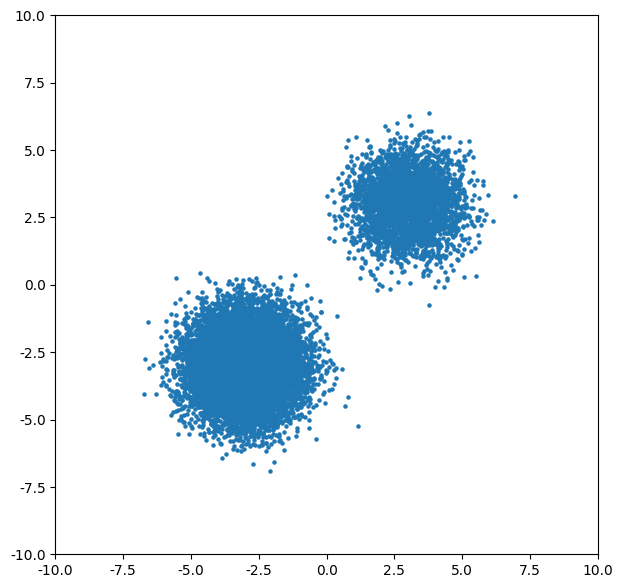
And after 1000 training iterations, here is the inference process looks like: we have N data points which are pure Gaussian noises. are now learned such that sampling from it can recover the original data distribution (although I feel the two distributions are not 8-2 in quantities):
Reference
([1] and [2] are good learning materials for me to write this post; [3] and [4] are good coding examples.)
[1] https://lilianweng.github.io/posts/2021-07-11-diffusion-models/
[2] https://aman.ai/primers/ai/diffusion-models/
[3] https://www.youtube.com/watch?v=a4Yfz2FxXiY
[4] https://github.com/JeongJiHeon/ScoreDiffusionModel#content–tutorial–blog-kr-