Back to the old days, I’ve studied how to implement highly efficient PyTorch pipelines for multi-gpu training [1]. DistributedDataParallel is the way to go, but it is cumbersome that we need boilerplates for spawning workers and constructing data readers.
Now, PyTorch Lighting offers clean API for setting up multi-gpu training easily. Here is a template I designed, which I will stick to for prototyping models for the rest of my life : )
import os
from typing import List, Any

from dataclasses import dataclass
import torch
import torch.distributed as dist
from torch import nn
from torch.nn import functional as F
from torch.utils.data import DataLoader, IterableDataset, random_split
from torchvision.datasets import MNIST
from torchvision import transforms
import pytorch_lightning as pl
from pytorch_lightning.metrics.functional import accuracy


TOTAL_NUM_BATCHES = 320
BATCH_SIZE = 32
STATE_DIM = 5
NUM_GPUS = 2
NUM_WORKERS = 2
UPDATE_FREQ = 1
WEIGHTS = torch.tensor([2.0, 3.1, 2.1, -1.5, -1.7])

@dataclass
class PolicyGradientInput:
    pid: int
    state: torch.Tensor
    reward: torch.Tensor

    def __len__(self):
        return self.state.shape[0]

    @classmethod
    def from_batch(cls, x):
        return cls(
            pid=x[0][0].item(),
            state=x[1][0].reshape(BATCH_SIZE, STATE_DIM),
            reward=x[2][0].reshape(BATCH_SIZE, 1),
        )

class EpisodicDataset(IterableDataset):
    def __iter__(self):
        worker_info = torch.utils.data.get_worker_info()
        pid = os.getpid()
        if worker_info is None:
            total_num_batches = TOTAL_NUM_BATCHES // NUM_GPUS
            worker_id = -1
        else:
            total_workers = worker_info.num_workers
            total_num_batches = int(TOTAL_NUM_BATCHES // NUM_GPUS // total_workers)
            worker_id = worker_info.id
        # You will see that we have an EpisodicDataset on each of NUM_GPUS processes
        print(f"{worker_info}, pid={pid}, total_num_batches={total_num_batches}")

        for _ in range(total_num_batches):
            state = torch.randn(BATCH_SIZE, STATE_DIM)
            reward = torch.sum(state * WEIGHTS, dim=1)
            yield (pid, state, reward)


class PPO(pl.LightningModule):
    def __init__(self):
        super().__init__()
        self.model = nn.Sequential(
            nn.Linear(STATE_DIM, 128), nn.ReLU(), nn.Linear(128, 128), nn.ReLU(), nn.Linear(128, 1)
        )
        self.traj_buffer = []
        self.update_freq = UPDATE_FREQ
        self.step = 0

    def training_step(self, batch: List[Any], batch_idx):
        batch: PolicyGradientInput = PolicyGradientInput.from_batch(batch)
        self.traj_buffer.append(batch)
        self.step += 1
        rank = dist.get_rank()
        # use first three trajectories' pids as as signature. quickly check if all trainers share the same data
        # the answer is each trainer maintains different trajectories
        traj_buffer_signature = ','.join([str(traj.pid) for traj in self.traj_buffer[:3]])
        print(f"rank={rank}, traj_buffer_len={len(self.traj_buffer)}, step={self.step}, signature={traj_buffer_signature}")
        if self.step % self.update_freq == 0:
            model_params = list(self.model.parameters())[0][0].detach().cpu().numpy()
            print(f"before {self.step} step training: rank={rank}, model_params={model_params}")
            return self.update_model()

    def configure_optimizers(self):
        # Somehow, Adam doesn't work for linear regression
        # optimizer = torch.optim.Adam(self.parameters(), lr=1e-2)
        optimizer = torch.optim.SGD(self.parameters(), lr=1e-2)
        return optimizer

    def update_model(self):
        traj = self.traj_buffer[-1]
        loss = F.mse_loss(self.model(traj.state), traj.reward)
        rank = dist.get_rank()
        print(f"rank={rank}, step={self.step}, loss={loss}")
        return loss


ds = EpisodicDataset()
dl = DataLoader(ds, batch_size=1, num_workers=NUM_WORKERS, pin_memory=True)
ppo = PPO()
trainer = pl.Trainer(gpus=NUM_GPUS, max_epochs=1, progress_bar_refresh_rate=1, accelerator='ddp')
trainer.fit(ppo, dl)
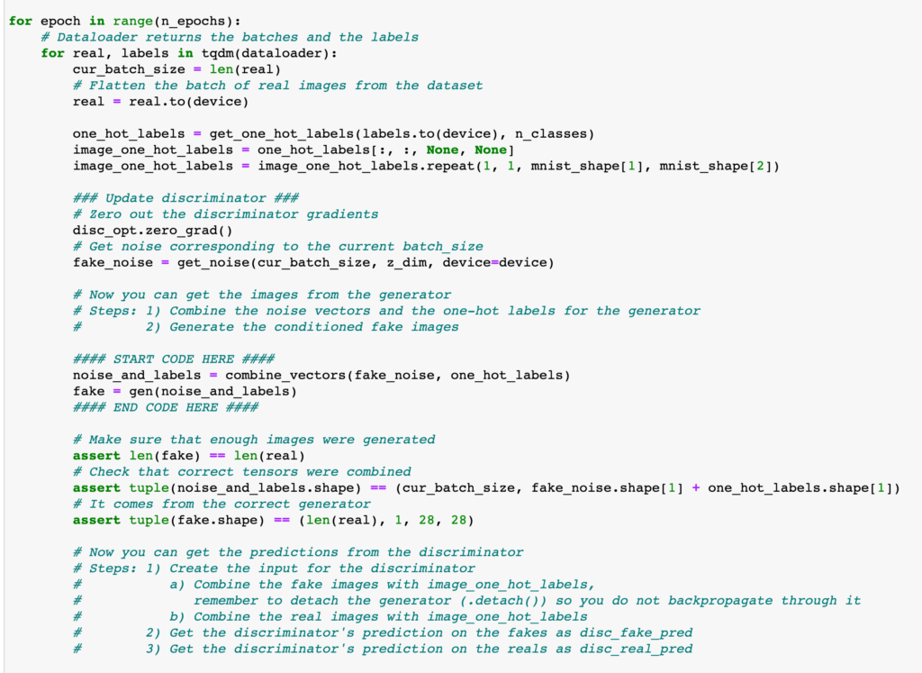
As you can see, you only need to define a Dataset, a DataLoader with appropriate NUM_WORKERS, and a pytorch-lightning Trainer in which you specify the number of gpus. Each of the NUM_GPUS GPUs will then use NUM_WORKERS processes for reading data and use one main process for training the model.
The example shows that each trainer on a GPU maintains a list of trajectories, which is not shared with the trainers on other GPUs. However, I believe model parameters are synced after every loss function computation because the underlying mechanism is still DistributedDataParallel.
References
[1] https://czxttkl.com/2020/10/03/analyze-distributeddataparallels-behavior/

 .
. 

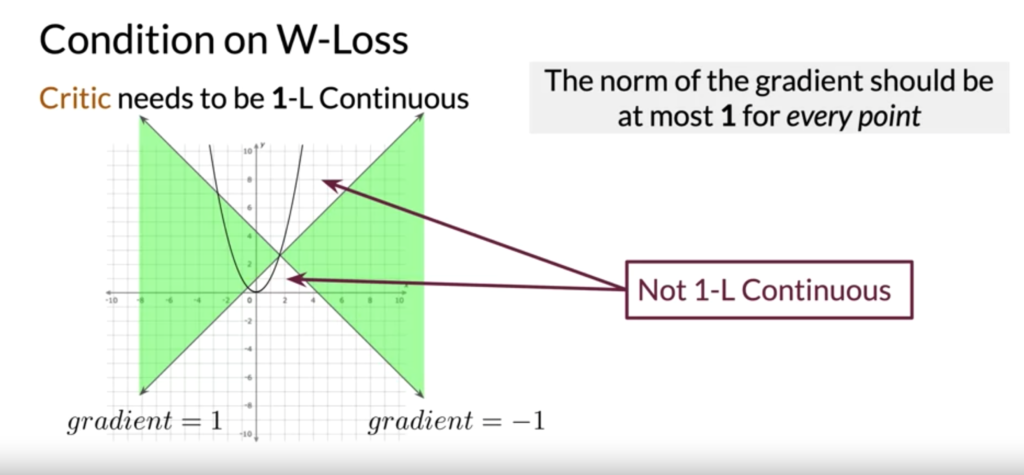
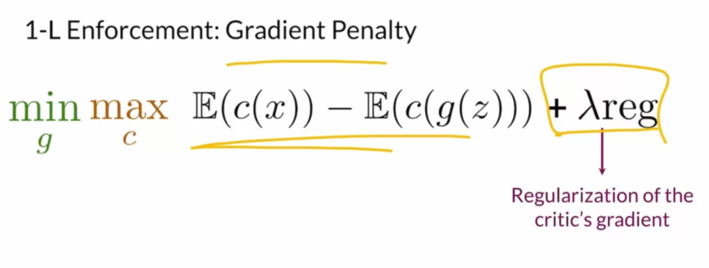
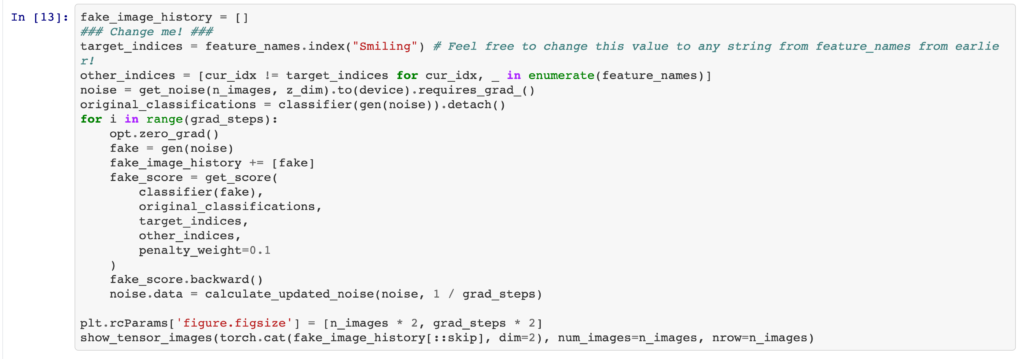
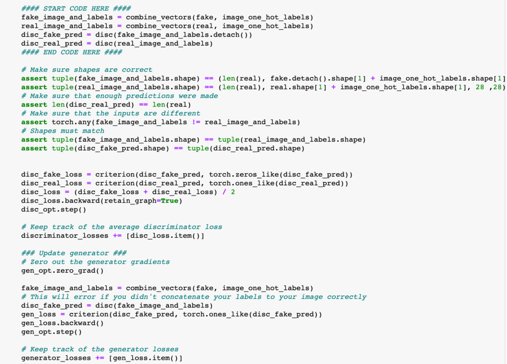
![max_g -\left[\mathbb{E}\left(log d(x)\right) +\mathbb{E}\left(1 - log d(g(z)) \right) \right]](https://czxttkl.com/wp-content/ql-cache/quicklatex.com-f94cdb5cdeb58b0480074930087633e2_l3.png "Rendered by QuickLaTeX.com") ) would provide little useful gradient when the discriminator is perfect in separating real and generated outputs. (There is much theory to dig in, but [4] gives a very well explanation on how it is superior in preventing mode collapsing and vanishing gradient.) The Wasserstein-loss approximates a better distance function than BCEloss called Earth Mover’s Distance which provides useful gradient even when the real and generated output is already separable.
) would provide little useful gradient when the discriminator is perfect in separating real and generated outputs. (There is much theory to dig in, but [4] gives a very well explanation on how it is superior in preventing mode collapsing and vanishing gradient.) The Wasserstein-loss approximates a better distance function than BCEloss called Earth Mover’s Distance which provides useful gradient even when the real and generated output is already separable.

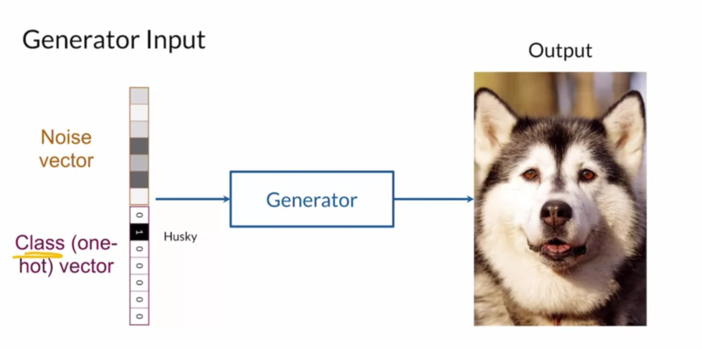
 takes as input a noise vector
  (as in the original GAN) and additionally, a latent code
  that learns semantic categories by unsupervised learning. A clever idea is proposed that the mutual information between
  and
and  should be maximized. In other words,
  should reveal as much information as possible about
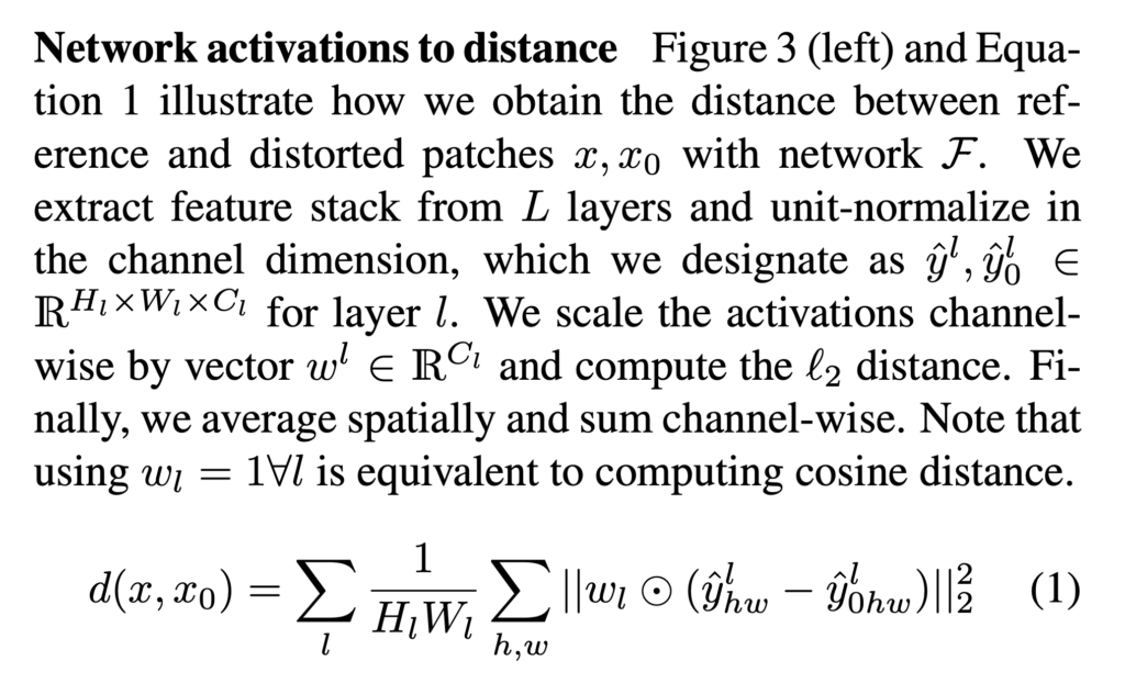
 layers of a pre-trained network. As shown in Eqn. 1 below, the distance between two images is a weighted sum of per-layer similarity. There is a learnable parameter
  in per-layer similarity, which is learned to optimize for differentiating more similar image pairs from less similar pairs. Eventually, LPIPS can be used to measure the distance between real and fake images in GAN.

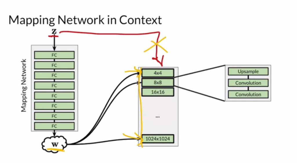
 vectors to different layers of the generator:
 to
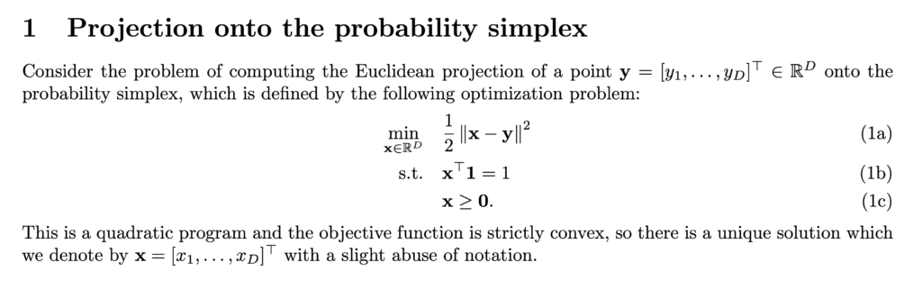
to  on the simplex. Since we often encounter problems of the sum-to-1 constraint, I think it is worth listing the solution in this post.
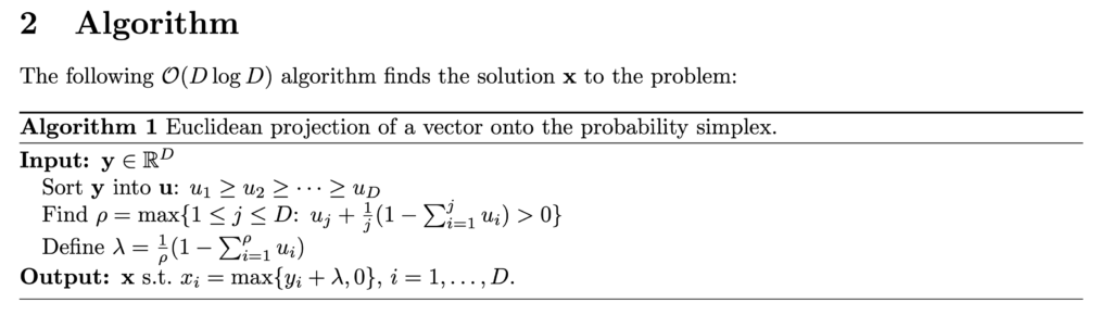
 can be understood as representing the (signed) volume of the parallelepiped transformed from an n-dimensional unit cube by
 and
and  (corresponding to
  , which is the definition of the determinant of
  on an
on an  -cardinality set
  is a probability distribution over the power set of
  ). Determinant point process represents a family of probability distributions such that for any subset
  , its probability density has a closed form as:
 matrix indexed by the elements of
  is an identity matrix of the same size, and
  is a sub-matrix of
 ![L_s \equiv [L_{ij}]_{i,j \in s}](https://czxttkl.com/wp-content/ql-cache/quicklatex.com-aa26ef8420ba9fff45fdeb156c38c7a1_l3.png "Rendered by QuickLaTeX.com") .
.
 , where
  has a size
  . Then, each column of
  ,
,  , which can be thought of as the normalized feature vector of one item in
  (
( ) scaled by a quality scalar
  . Next, as we know that
  and
and  , we know that
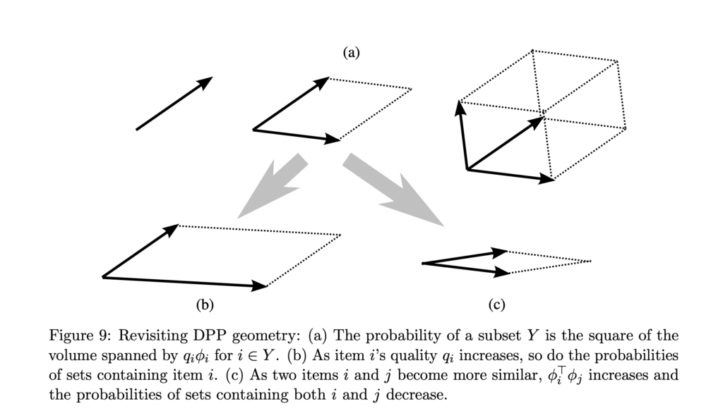
  . The volume of the parallelepiped characterized by
  is affected by both
  . The larger the
  (for any
  ) is, the more similar the two items are, and consequently the smaller the volume is. This can be best understood in when
  or
or  :
: 
 as the best subset of
  . Now we introduce a concept:
  . Then
  is submodular because
  for any
  . Intuitively, adding elements to
  ). Submodular maximization is NP-hard (i.e., can be reduced to an NP problem in polynomial time). (But interestingly, submodular minimization can be solved exactly in polynomial time, see introduction in Section 1.2.1 in one’s
 is an item candidate set,
  is each item’s category (one-hot vector),
  is the score of each item, and
  is a utility vector for governing the total utility of the final selected item set. The optimal item set will optimize
  . And in practice it is optimized by a greedy method.
 , where
  is the feature vector and
  is a binary label, a model predicts
  . Then the cross entropy function can be expressed as:
![\[CE(p,y)=-ylog(p)-(1-y)log(1-p)\]](https://czxttkl.com/wp-content/ql-cache/quicklatex.com-7baa6ecc974f172aed9465e931bd93e9_l3.png "Rendered by QuickLaTeX.com")
 if
if  or
or  if
if  , then
  , as shown in the blue curve below:
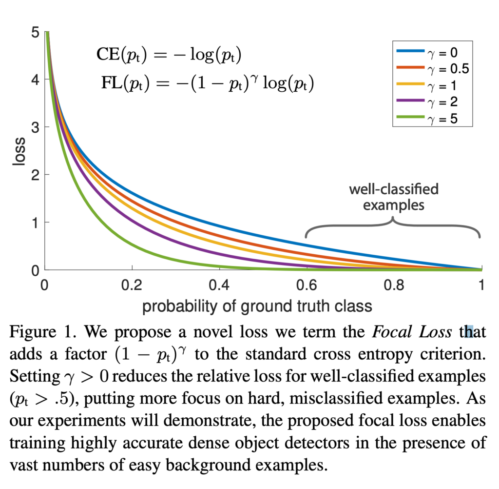
 . By tuning with different
  ‘s, you can see that the loss curve gets modulated differently and easy examples’ loss become less and less important.
 being the absolute prediction. error:
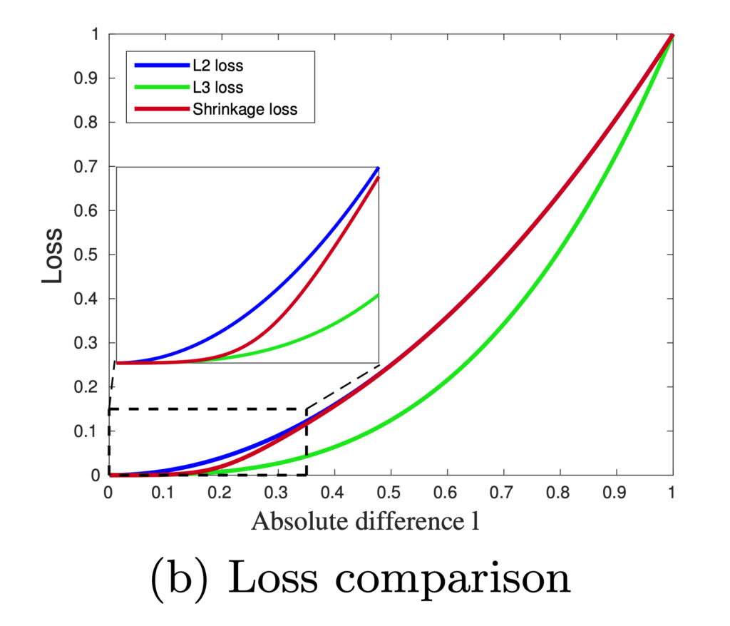
![\[L_2 = | p - y |^2 = l^2\]](https://czxttkl.com/wp-content/ql-cache/quicklatex.com-f80ece0e582297fc6c50085a3e275683_l3.png "Rendered by QuickLaTeX.com")
![\[FL\_L_2=l^\gamma \cdot l^2 = l^{\gamma+2}\]](https://czxttkl.com/wp-content/ql-cache/quicklatex.com-d2b33f6ef1483fe55c37156838aaa028_l3.png "Rendered by QuickLaTeX.com")
 by letting
  penalty effective almost only on the easy examples but not on the hard examples. They call it the shrinkage loss:
![\[L_S = \frac{l^2}{1 + exp\left(a\cdot \left( c-l \right)\right)}\]](https://czxttkl.com/wp-content/ql-cache/quicklatex.com-60f04910d6082a4a6a347f51491eeac0_l3.png "Rendered by QuickLaTeX.com")
 on
on  but there is some unobserved confounding factor that may impede your estimation (i.e., you can’t directly do
  regression). So we can introduce an instrument variable
  is some hidden confounding factor that may affect
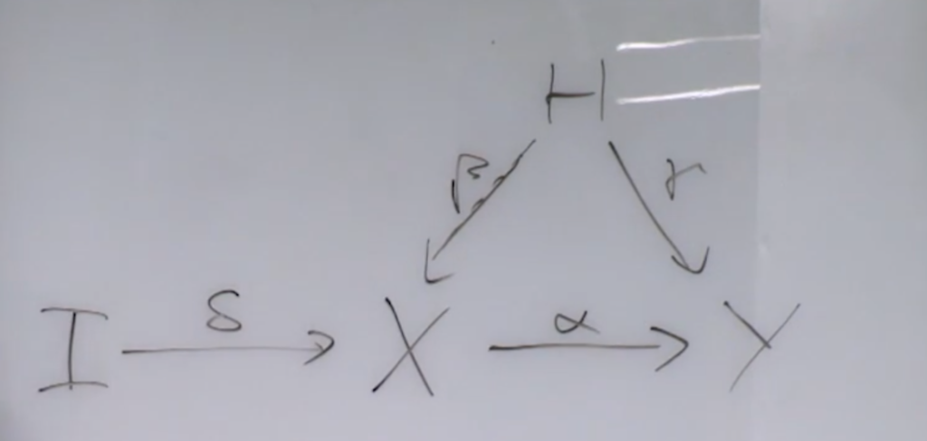


 without depending on
  . Then using the fitted value of
  , we regress
  . The coefficient learned that is associated with
  in
in  .
. 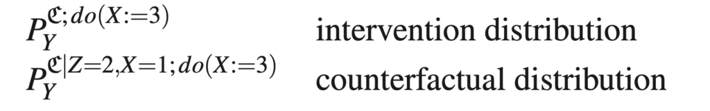
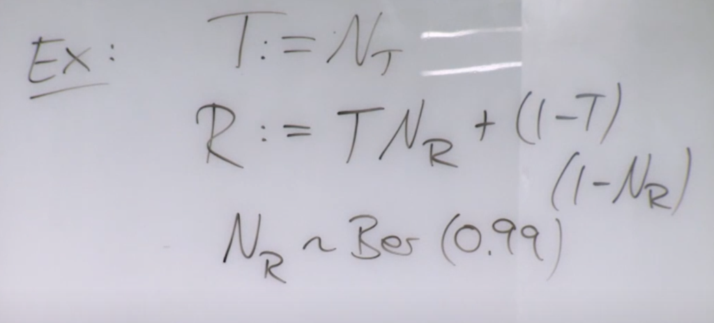
 is a treatment to a disease.
  is the recovery result, which depends on whether one receives the treatment and a noise
  following a Bernoulli distribution. According to the provided structural causal model (SCM), the intervention distribution of
  would be
  . Note that this specific patient has a new SCM:
  ,
,  . The counterfactual distribution
  on the old SCM would be the same as the intervention distribution on the new SCM.
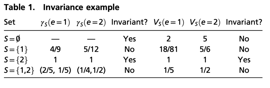
 . The core assumption of causal invariant prediction is that in a SCM and any inventional distribution based on it,
  remains invariant if the structural equation for
  for every feature subset
  for each SCM. Across different SCMs, we would find all
  . Then the parent of