Many ways towards recommendation diversity

Diversity of recommendations keeps users engaged and prevents boredom [1]. In this post, I will introduce several machine learning-based methods to achieve diverse recommendations. The literature in this post is mostly retrieved from the overview paper “Recent Advances in Diversified Recommendation” [6].

Determinant Point Process

Let’s first review what is the determinant of a matrix [2]. The determinant of matrix $A$ can be understood as representing the (signed) volume of the parallelepiped transformed from an n-dimensional unit cube by $A$ . The parallelepiped is defined by the vertices of coordinates same as $A$ ‘s column vectors. Let’s look at a 2D example:

(1) $\begin{align*}|A| = \begin{vmatrix} a & b\\c & d \end{vmatrix}=ad - bc \end{align*}$

$A$ transforms a unit square on the 2D plane to a parallelogram characterized by two vertices $(a,c)$ and $(b,d)$ (corresponding to $A$ ‘s first column and second column). Therefore, according to basic math [3], this parallelogram’s area can be computed as $ad - bc$ , which is the definition of the determinant of $A$ .

A point process $\mathcal{P}$ on an $N$ -cardinality set $S$ is a probability distribution over the power set of $S$ (i.e., $2^{N}$ ). Determinant point process represents a family of probability distributions such that for any subset $s \subseteq S$ , its probability density has a closed form as:

(2) $\begin{align*}P(s \subseteq S)=\frac{det(L_s)}{det(L+I)} \propto det(L_s),\end{align*}$

where $L$ is a constructed $N\times N$ matrix indexed by the elements of $S$ , $I$ is an identity matrix of the same size, and $L_s$ is a sub-matrix of $L$ : $L_s \equiv [L_{ij}]_{i,j \in s}$ .

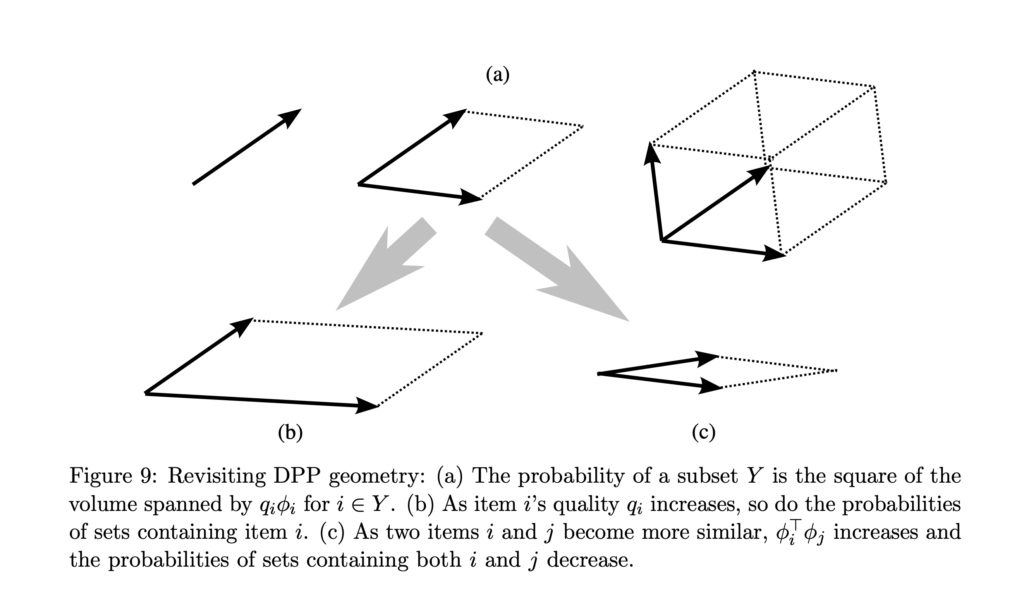
$L$ can be constructed in a way to give the determinant point process a beautiful interpretation on balancing individual items’ quality and inter-item diversity. First, we can rewrite $L$ as a Gram matrix: $L=B^T B$ , where $B$ has a size $K \times N$ . Then, each column of $B$ can be represented as $B_i=q_i \dot \phi_i$ , $i=1,\dots,N$ , which can be thought of as the normalized feature vector of one item in $s$ ( $\Vert\phi_i \Vert_2=1$ ) scaled by a quality scalar $q_i$ . Next, as we know that $P(s \subseteq S) \propto det(L_s)$ and $det(AB)=det(A)det(B)$ , we know that $det(L_s)=det^2(B)=Vol\_of\_Parallelepiped^2(\{B_i\}_{i\in s})$ . The volume of the parallelepiped characterized by $\{B_i\}_{i\in s}$ is affected by both $q_i$ and $\phi_i$ . The larger the $q_i$ is, the larger the volume. The larger $<\phi_i, \phi_j>$ (for any $i,j\in s$ ) is, the more similar the two items are, and consequently the smaller the volume is. This can be best understood in when $|s|=2$ or $3$ :

We denote $s^*$ as the best subset of $S$ that can achieves the highest $P(s \subseteq S)$ . Now we introduce a concept: $P(s \subseteq S)$ is log-submodular (Section 2.2 in [7]). Suppose $f(s)=log P(s \subseteq S)$ . Then $f(s)$ is submodular because $f(s \cup i) - f(s) \geq f(s' \cup i) - f(s')$ for any $s \subseteq s' \subseteq S \setminus \{i\}$ . Intuitively, adding elements to $s$ yields diminishing returns in $f(s)$ as $s$ is getting large. As [5] reveals (around Eqn. 74), $f(s)$ is also non-monotone, as the additional of even a single element can decrease the probability. Submodular maximization corresponds to finding $s^*$ that has the highest $P(s \subseteq S)$ (or $log P(s \subseteq S)$ ). Submodular maximization is NP-hard (i.e., can be reduced to an NP problem in polynomial time). (But interestingly, submodular minimization can be solved exactly in polynomial time, see introduction in Section 1.2.1 in one’s thesis). Therefore, in practice, we turn to approximate method for $P(s \subseteq S)$ maximization. [4] introduces one simple greedy algorithm (Eqn. 15).

Simple Submodular Diversification

Before DPP is introduced to solve the diversification problem, Amazon has proposed a simpler idea to model diversification [9], which is also one kind of submodular minimization.

Here, $\mathcal{A}_k$ is an item candidate set, $\mathbf{a}_i$ is each item’s category (one-hot vector), $s(\mathbf{a}_i)$ is the score of each item, and $\mathbf{w}$ is a utility vector for governing the total utility of the final selected item set. The optimal item set will optimize $\pho$ . And in practice it is optimized by a greedy method. $\mathbf{w}$ is the only learnable parameter of the same dimension as the number of categories. If we want to learn a global optimal $\mathbf{w}$ , we will need to estimate each category’s CTR by bayesian probability. If we want to learn a personalized $\mathbf{w}$ , we will need to estimate each user’s CTR on each category.

Calibrate recommendation to user history

[8] introduces another idea of doing calibration. The tenet of it is that the recommended list should have similar topic distributions as the user watched history. You can look at Section 3 of [8] to get the exact formula. Basically, they use KL-divergence to measure the difference between the recommendation and user history.