czxttkl

New progress of generative modeling – flow matching

In a previous post, we discussed an earlier generative modeling called Normalizing Flows [1]. However, Normalizing Flows has its own limitations: (1) it requires the flow mapping function $f(x)$ to be invertible. This limits choices of potential neural network architectures to instantiate $f(x)$ , because being invertible means that hidden layers must have the exact same dimensionality as the input. (2) computing the log⁡ of determinant of the jacobian matrix of $f(x)$ is expensive, usually in $O(N^3)$ time complexity.

Flow matching is a more recent developed generative modeling technique with lower training cost (see the comparison between Normalizing Flows vs Flow Matching in [2] and a more mathematical introduction of how Flow Matching evolved from Normalizing Flows [6]). In this post, we are going to introduce it. Two materials help me understand flow matching greatly: (1) neurips flow matching tutorial [3] (2) an MIT teaching material [4]

Flow Matching

Motivation

We start from the motivation. Suppose $\mathbb{R}^d$ represents the target space we want to generate (e.g., all dog pictures with $d$ representing the image dimension). The goal of generative modeling is to learn the real target distribution $q$ . To enable generating different targets stochastically, the goal usually becomes to learn the transformation from an initial random distribution $p$ (e.g., Gaussian) the real data distribution $q$ .

A straightforward method is GAN [5]. However, GAN faces various training instability issues and cannot give the likelihood of a data point, while Flow Matching can address both pain points.

Ordinary Differential Equations (ODE)

ODE describes how a system changes over time. An ODE is defined as:

$\begin{align*} \frac{d}{dt} X_t &= \mu_t(X_t) \\ X_0&=x_0, \end{align*}$

where $X: [0, 1] \rightarrow \mathbb{R}^d$ . In natural language, we say that $X_t$ is a variable representing any point in the $d$ -dimensional system at time $t$ , where each dimension is between 0 and 1. At a given time $t$ ( $t$ is also between 0 and 1), $X_t$ should move in the direction of $\mu_t(X_t)$ , which we call the velocity. $\mu_t(X_t)$ is also a $d$ -dimensional vector. The solution of an ODE is called flow, $\psi_t(x_0)$ , which tells you where an initial point will be at time $t$ . Hence $\psi_t(x_0)$ ‘s input is an $d$ -dimensional point and output is also an $d$ -dimensional point. The ODE above can be rewritten with $\psi_t(x_0)$ :

$\begin{align*} \frac{d}{dt} \psi_t(x_0) &= \mu_t(\psi_t(x_0)) \\ \psi_0(x_0)&=x_0, \end{align*}$

The example below shows how a system moves – the red square grid is the flow, describing each initial point’s “landing” point at time $t$ , and the blue arrow is the velocity at time $t$ .

The goal of flow matching is to learn a velocity function $\mu_t^\theta(x)$ such that $X_0 \sim p_{init}$ and $X_1 \sim p_{data}$ . With a known/learned velocity function, you can easily simulate how the system changes, which is equivalent to the flow function $\psi_t(x_0)$ :

Conditional / Marginal Probability Path, Conditional and Marginal Velocity Fields

This section is the most mathematical-heavy one. We first introduce the concept of conditional probability path, $p_t(x|z)$ . In natural language, $p_t(x|z)$ means the distribution of the position of a point at time $t$ if that point starts from $p_{init}$ at time 0 and ends at exactly $z$ (i.e., a delta distribution at $z$ ) at time 1, where $z$ is any data sampled from the target distribution $p_{data}$ . Therefore, the marginal probability path $p_t(x)$ can be described as:
$p_t(x)=\int p_t(x|z)p_{data}(z)dz$ .
$p_t(x)$ simply describes the position distribution of the whole system at time $t$ , given the initial distribution is $p_{init}$ and the end distribution is $p_{data}$ .

The diagram below describes an example of conditional probability path $p_t(x|z)$ : it starts from a 2D gaussian distribution and ends at a particular position marked by the red dot.

The diagram below describes an example of marginal probability path $p_t(x)$ : it starts from a 2D gaussian distribution and ends at a chessboard-patterned distribution.

Deriving from the concepts of conditional/marginal probability path, we can also have conditional and marginal velocity field, defined as:
Conditional velocity field: $X_0 \sim p_{init}, X_t\sim p_t(\cdot|z) \; (0 \leq t \leq 1) \Rightarrow \frac{d}{dt} X_t = \mu_t(X_t|z)$
Marginal velocity field: $\mu_t(x) = \int \mu_t(x|z) \frac{p_t(x|z) p_{data}(z)}{p_t(x)} dz$

The formula of marginal velocity field needs a bit work to be proved. We use the rest of this section to prove that.

First, we introduce a theorem called Continuity Equation:

where the divergence operator is defined as:

In natural language, this equation says that the change of marginal probability path w.r.t. time is equal to the negative divergence of $p_t(x) \cdot \mu_t(x)$ . The same theorem can also be applied to the conditional probability path: $\partial_t p_t(x|z) = -div\left(p_t(\cdot|z)\mu_t(\cdot|z)\right)(x)$ .

Now we can show that:

$\begin{align*} \partial_t p_t(x) &= \partial_t \int p_t(x|z)p_{data}(z) dz\\ &=\int \partial_t p_t(x|z)p_{data}(z) dz \\ &=\int -div\left( p_t(\cdot|z)\mu_t(\cdot|z) \right)(x) p_{data}(z) dz \\ &=-div \left( \int p_t(x|z) \mu_t(x|z) p_{data}(z)dz\right)(x) \\ &=-div \left( p_t(x)\int \mu_t(x|z) \frac{p_t(x|z) p_{data}(z)}{p_t(x)}dz\right)(x) \\ &=-div\left( p_t \mu_t \right)(x) \qquad \text{(by definition)} \end{align*}$

By the last two equations, we proved the relationship between the marginal and conditional velocity fields: $\mu_t(x) = \int \mu_t(x|z) \frac{p_t(x|z) p_{data}(z)}{p_t(x)} dz$

Training a Practical Flow Matching model

To reiterate the motivation of flow matching: our goal is to learn a velocity function $\mu_t^\theta(x)$ such that $X_0 \sim p_{init}$ and $X_1 \sim p_{data}$ . Therefore, the ultimate goal should be:
$\mathcal{L}_{FM}(\theta) = \mathbb{E}_{t\sim Unif[0,1], x\sim p_t} \left[ \left\Vert \mu_t^\theta(x)-\mu_t(x) \right\Vert^2 \right] = \mathbb{E}_{t\sim Unif[0,1], z\sim p_{data}, x\sim p_t(\cdot|z)} \left[ \left\Vert \mu_t^\theta(x)-\mu_t(x) \right\Vert^2 \right]$

Recall in the section above that $\mu_t(x) = \int \mu_t(x|z) \frac{p_t(x|z) p_{data}(z)}{p_t(x)} dz$ , which involves an integration operator and thus is intractable. Interestingly, we can prove that $\mathcal{L}_{FM}(\theta)=\mathbb{E}_{t\sim Unif[0,1], z\sim p_{data}, x\sim p_t(\cdot|z)} \left[ \left\Vert \mu_t^\theta(x)-\mu_t(x) \right\Vert^2 \right] = \mathbb{E}_{t\sim Unif[0,1], z\sim p_{data}, x\sim p_t(\cdot|z)} \left[ \left\Vert \mu_t^\theta(x)-\mu_t(x|z) \right\Vert^2 \right] = \mathcal{L}_{CFM}(\theta)$ . Therefore, we can explicitly regress our parameterized velocity function against a tractable conditional vector field. This proof can be found in Theorem 18 in [4].

The exact form of $\mu_t(x|z)$ depends on what family of probability path we choose. One particularly popular probability path is the Gaussian probability path. We can define $\alpha_t$ and $\beta_t$ to be two continuously differentiable, monotonic functions with $\alpha_0=\beta_1=0$ and $\alpha_1=\beta_0=1$ . We can verify that the conditional Gaussian probability path parameterized by $\alpha_t$ and $\beta_t$ , $p_t(\cdot|z)=\mathcal{N}(\alpha_tz, \beta_t^2 I_d)$ , satisfies the definition of a conditional probability path: at time 0, $p_0(\cdot|z) = \mathcal{N}(\alpha_0 z, \beta_0^2 I_d) = \mathcal{N}(0, I_d)$ and $p_1(\cdot|z) = \mathcal{N}(\alpha_1 z, \beta_1^2 I_d) = \delta_z$ . Note that, with the Gaussian conditional probability path, we can simulate the position of $x_t$ : $x_t = \alpha_t z + \beta_t \epsilon$ , where $\epsilon \sim \mathcal{N}(0, I_d)$ . We can then prove that $\mu_t(x|z)=\left(\dot{\alpha_t}-\frac{\dot{\beta_t}}{\beta_t}\alpha_t \right)z + \frac{\dot{\beta_t}}{\beta_t}x$ (see detailed proof in Example 11 in [4]).

With all these intermediate artifacts, we can derive the loss function:

$\begin{align*} \mathcal{L}_{CFM}(\theta) &= \mathbb{E}_{t\sim Unif[0,1], z\sim p_{data}, x\sim p_t(\cdot|z)} \left[ \left\Vert \mu_t^\theta(x)-\mu_t(x|z) \right\Vert^2 \right] \\ &= \mathbb{E}_{t\sim Unif[0,1], z\sim p_{data}, x\sim p_t(\cdot|z)} \left[ \left\Vert \mu_t^\theta(x)-\left(\dot{\alpha_t}-\frac{\dot{\beta_t}}{\beta_t}\alpha_t \right)z - \frac{\dot{\beta_t}}{\beta_t}x \right\Vert^2 \right] \\ &(\text{let } x=\alpha_t z + \beta_t \epsilon) \\ &= \mathbb{E}_{t\sim Unif[0,1], z\sim p_{data}, x\sim p_t(\cdot|z)} \left[ \left\Vert \mu_t^\theta(\alpha_t z + \beta_t \epsilon) - (\dot{\alpha_t} z + \dot{\beta_t} \epsilon) \right\Vert^2 \right] &(\text{special case: } alpha_t=t, \beta_t=1-t) \\ &=\mathbb{E}_{t\sim Unif[0,1], z\sim p_{data}, x\sim p_t(\cdot|z)} \left[ \left\Vert \mu_t^\theta(tz+(1-t)\epsilon) - (z- \epsilon) \right\Vert^2 \right] \end{align*}$

References

[1] https://czxttkl.com/2021/11/15/normalizing-flows/

[2] https://medium.com/@noraveshfarshad/flow-matching-and-normalizing-flows-49c0b06b2966

[3] https://neurips.cc/virtual/2024/tutorial/99531

[4] https://diffusion.csail.mit.edu/docs/lecture-notes.pdf

[5] https://czxttkl.com/2020/12/24/gan-generative-adversarial-network/

[6] https://mlg.eng.cam.ac.uk/blog/2024/01/20/flow-matching.html

Learn GPU Optimization

It has been a while since I learned GPU knowledge. I am going to keep updating more recent materials for ramping up my GPU knowledge.

FlashAttention [1]

We start from recapping the standard Self-Attention mechanism, which is computed in 3-passes:
$Q, K, V \in \mathbb{R}^{N \times d}$
$S = QK^T \;\;\quad shape=(N \times N)$
$P=softmax(S)\;\;\quad shape=(N \times N)$
$O=PV\;\;\quad shape=(N \times d)$

Notes:

The shape $N$ and $d$ represent the sequence length and internal dimension, respectively. $Q=W_k X$ , $K=W_k X$ , $V=W_v X$ , which transform token embeddings $X$ into a projected latent space.
$P$ is the attention matrix. $P_{i,j}$ represents how much attention token $i$ should pay for $j$ . In normal LLM tasks, we will apply a causal mask so that only $P_{i,j} \;(i>j)$ is valid, because a token can only pay attention to all previous tokens. The softmax() operator is applied per-row of $S$ .
The output $O$ represents the weighted values from other tokens per position. $O$ will be fed to feed forward layers to be transformed into output space (from shape $(N\times d)$ to $(N \times {vocab\_size})$ ). We omit the part after self-attention.

How GPUs work is that GPUs have a massive number of threads to execute an operation (called a kernel). Each kernel loads inputs from HBM to registers and SRAM, computes, then writes outputs to HBM. HBM has larger storage but slower speed. In practice, the times of HBM accesses play a non-negligible role in GPU execution speed. In standard self-attention, it requires $O(Nd+N^2)$ HBM accesses, because we need to load $Q$ , $K$ , and $V$ from HBM and we need to read/write of $S$ and $P$ , each of shape $(N\times N)$ . A detailed breakdown of standard self-attention HBM accesses is as below (illustrated by Gemini): Let’s dive into the step of computing softmax. Even computing softmax has many details. First, in real world, we usually need to compute a safe softmax version, where we subtract each input to the softmax with the maximum input to avoid potential overflow. (Diagrams from [3]) In its vanilla implementation, we need to have three passes: the first pass computes the maximum of the input, the second pass computes the denominator of the softmax, and the third pass computes the actual softmax. Asymptotically these three steps require $O(N^2)$ time but in reality the constant factor of the $N^2$ computation is also important. SRAM is typically too small to hold the $N^2$ -size $S=QK^T$ result. So we either need to save $S$ into HBM in the first pass and load it in the following two steps, or even need to recompute $QK^T$ , depending whichever is faster. That means this three-passes safe softmax algorithm does require $3N^2$ computation time / accesses to HBM. It turns out that we can turn the 3-passes algorithm into 2-passes. This is something called online softmax. As we traverse each $x_i$ , we can record the maximum value so far and the accumulative softmax denominator. The accumulative softmax denominator from the previous $x_{i-1}$ can be easily scaled whenever a new maximum is found at $x_i$ . With this 2-pass online softmax algorithm, self-attention can also be computed in two-passes: However, we can do better by finding that $\mathbf{o}_i$ can also be computed “online” together with the running maximum value $m_i$ and running accumulative softmax denominator $d_i'$ . That’s how we end up with FlashAttention which requires one pass to compute the output vectors! In reality, a further optimization is to load Q/K/V in blocks so that the blocks of Q, K, V, and O can occupy roughly the full SRAM memory at one time. That’s why we see block size is set at $B_c=\lceil \frac{M}{4d} \rceil$ or $B_r=min\left( \lceil \frac{M}{4d}\rceil, d\right)$ in the algorithm. Now, we examine how to do backward computation in FlashAttention. We start from examining the standard attention backward pass: (To clarify the notations, $dO$ is the gradient of the loss $\mathcal{L}$ with respect to the attention output matrix, i.e., $dO=\frac{\partial L}{\partial O}$ , which has the same shape as $O$ . Similarly for $dQ$ , $dK$ , and $dV$ . We also assume $dO$ is already available as the backpropagation computation has been done from $\mathcal{L}$ to $O$ ) Let’s try to understand this standard backward pass:

With $O = PV$ , due to matrix calculus rules, we have $dV = P^T dO$ .
We need to compute and record $dP$ because it will be used in computing $dQ$ and $dK$ . Due to matrix calculus rules, we have $dP=dO V^T$ .
$dS = \frac{\partial L}{\partial S}= \frac{\partial L}{\partial P} \frac{\partial P}{\partial S}$ . There is a well-known mathematical result stating that the Jacobian matrix of softmax can be computed by $J(P_i) = J\left(softmax(S_i)\right)=\left[ \frac{\partial P_i}{\partial s_{i1}}, \cdots, \frac{\partial P_i}{\partial s_{iN}} \right]=diag(P_i) - P_i P_i^T$ , where $P_i$ is a row of $P$ . With some simplification, we reach to $d S_i = d P_i^T J(P_i)= P_i \odot dP_i - \left(dP_i^T P_i\right) \cdot P_i$ . [Note: while $P_i$ is a row of $P$ (and $dP_i$ is a row of $dP$ ), it is still treated a column vector following the convention of linear algebra. So $\left(dP_i^T P_i\right)$ is actually a scalar, an inner product, while $P_i P_i^T$ is a matrix, an outer product, of the two vectors.]
With $S=QK^T$ and matrix calculus rules, we obtain $dQ=dSK$ and $dK=dS^T Q$ .

As we can see, the standard attention backward pass requires loading $Q$ , $K$ , $V$ , $dO$ , $dS$ , $P$ , $dP$ and writing $dS$ , $dP$ , $dQ$ , $dV$ , and $dK$ . However, in FlashAttention we do not store $P$ . So in its backward pass, we also need to compute (blocks of) $P$ on the fly. Moreover, $dP_i^T P_i$ can be computed and prestored in HBM via $dO_i$ and $O_i$ :

(1) $\begin{align*} dP_i^T P_i &= (dO_i^T V^T) P_i \\ &=dO_i^T (V^T P_i) \\ &=dO_i^T (P_i^T V)^T \\ &=dO_i^T O_i \end{align*}$

Now let’s summarize IO complexity (i.e., HBM accesses) for standard attention and FlashAttention.

Forward pass:
1. standard attention: $O(Nd+N^2)$ as discussed above
2. FlashAttention: $O(N^2 d^2 M^{-1})$ because one full inner loop (starting from line 7 in Algorithm 1) needs to load the full $Q$ from HBM ( $O(Nd)$ ), and the outer loop (line 5 in Algorithm 1) needs to perform $T_c$ times ( $O(NdM^{-1})$ ). Another good reference of IO complexity analysis can be found in [4]
Backward pass:
1. standard attention: $O(Nd+N^2)$
2. FlashAttention: $O(N^2 d^2 M^{-1})$ Please see analysis in Theorem 5 in [1]

In practice, when will FlashAttention outperform Attention? This is when $d^2$ can be greatly smaller than $M^{-1}$ . First of all, we need to clarify that $M$ should represent the L1 cache size of one streaming multiprocessor (SM) in a GPU. Taking A100 as an example, one SM has 192KB L1 cache. So FlashAttention will probably have advantage of IO complexity when $d=$ 64, 128, or 256 but has no advantage when $d \geq 512$ . Let’s also summarize the total memory footprint required by standard attention vs FlashAttention: 1. standard attention: it needs to store $K$ , $V$ , and $O$ matrices, which needs $O(Nd)$ space. However the most costly part comes from storing $P$ and $S$ , which takes $O(N^2)$ space. Overall, the memory footprint is $O(Nd+N^2)$ . 2. FlashAttention: it still needs to store $K$ , $V$ , and $O$ matrices, which needs $O(Nd)$ space. But it does not store $P$ and $S$ ; instead it maintains the running maximum values and running accumulative softmax denominators in the forward pass so that they can be used in the backward pass, which takes $O(N)$ space. Overall, the memory footprint of FlashAttention is only $O(Nd)$ .

Now let’s move on to the engineering test. I picked one simple online implementation of FlashAttention and compared it with pytorch scaled dot product attention implementation (with backend=memory efficient) and a naive implementation of attention. Note that FlashAttention can be thought as a combination of reducing memory as HBM accesses. The pytorch implementation with the memory efficient backend essentially only reduces the memory footprint but not HBM accesses. The comparing script is here (python benchmark_flash_triton.py).

The comparison result is shown below. The numbers are TFlops measured. We test both forward and backward passes under the setting: num_heads = 48 and num_dim = 64. When OOM arises, we mark the result as -1. We can see the FlashAttention version clearly has higher FLOPs and can handle much longer sequences than the other two versions.

As a technique to reduce memory footprint and HBM accesses, FlashAttention is useful in training and the pre-filling stage in inference, both requiring obtaining the attention outputs of given sequences. So FlashAttention can be helpful to reduce time-to-first-token (TTFT). However, for the actual decoding phase, we need more pecialized variants (like Flash-Decoding). We will cover it later.

Torch.compile / CudaGraph

Cuda Graphs is an NVIDIA hardware-level optimization designed to speed up communication delay between CPU and GPU because sometimes your computation speed may be bottlenecked by how fast CPU sends kernel launch commands to GPU. The Cuda Graphs technique captures the kernel launch sequences in a graph structure first and then in the replay phase the CPU can just send one single command to GPU to execute the graph, which consists of all recorded kernel launches. Torch.compile is a set of optimization techniques that can be automatically applied to python+pytorch functions. It records python code logics in computation graphs and then rely on TorchInductor to conduct optimizations:

fuse operations/kernels
auto-tune kernel configurations like block sizes
Choose different backends for matmul and perform prologue and epilogue fusion (TODO: understand these fusions)
use CUDA Graphs to cache and replay kernel launches efficiently

As you can see, torch.compile is a superset of optimization techniques like Cuda Graphs. Below, we show a very basic example of how torch.compile accelerates a function. We test two modes of torch.compile, “max-autotune” and “max-autotune-no-cudagraphs”. While max-autotune gives torch.compile the full autonomy to compile your function, sometimes it may over-engineer it. For example, applying cuda graphs may be overkill for small functions like the one in the example below.

import torch
import time
import torch._dynamo as dynamo

# Ensure you have a CUDA-enabled GPU for the best results
device = 'cuda' if torch.cuda.is_available() else 'cpu'
print(f"Using device: {device}")

# 1. Define a simple function with a loop
def my_function(x):
    for _ in range(10):
        # A series of simple operations
        x = torch.sin(x) + torch.cos(x)
    return x

# 2. Create some input data
input_tensor = torch.randn(1024, 1024, device=device)

# 3. Compile the function
# The 'mode' can be tuned for different trade-offs. 'max-autotune' is aggressive.
compiled_function = torch.compile(my_function, mode="max-autotune")

# 4. Compile the function without cuda graph
# The 'mode' can be tuned for different trade-offs. 'max-autotune' is aggressive.
compiled_function_no_cuda_graph = torch.compile(my_function, mode="max-autotune-no-cudagraphs")

# --- Benchmarking ---

# WARM-UP RUNS: The first run has a one-time compilation overhead.
# We run both once to get this out of the way for fair timing.
print("\nStarting warm-up runs...")
_ = my_function(input_tensor)
_ = compiled_function(input_tensor)
_ = compiled_function_no_cuda_graph(input_tensor)
if device == 'cuda':
    torch.cuda.synchronize()
print("Warm-up complete.")


# Time the original EAGER mode function
print("\nBenchmarking Eager Mode...")
start_time = time.perf_counter()
for _ in range(100):
    _ = my_function(input_tensor)
# Make sure all GPU operations are finished before stopping the timer
if device == 'cuda':
    torch.cuda.synchronize()
eager_time = time.perf_counter() - start_time


# Time the COMPILED function
print("Benchmarking Compiled Mode...")
start_time = time.perf_counter()
for _ in range(100):
    _ = compiled_function(input_tensor)
if device == 'cuda':
    torch.cuda.synchronize()
compiled_time = time.perf_counter() - start_time


# Time the COMPILED function with no cuda graph
print("Benchmarking Compiled Mode with no Cuda Graphs...")
start_time = time.perf_counter()
for _ in range(100):
    _ = compiled_function_no_cuda_graph(input_tensor)
if device == 'cuda':
    torch.cuda.synchronize()
compiled_time_no_cuda_graph = time.perf_counter() - start_time


# --- Results ---
print("\n--- Results ---")
print(f"Eager mode total time:    {eager_time:.4f} seconds")
print(f"Compiled mode total time: {compiled_time:.4f} seconds")
print(f"Compiled mode with no cuda graph total time: {compiled_time_no_cuda_graph:.4f} seconds")
print(f"\nSpeedup: {eager_time / compiled_time:.2f}x faster! 🎉")
print(f"Speedup with no cuda graph: {eager_time / compiled_time_no_cuda_graph:.2f}x faster! 🎉")


# Use explain to see how Dynamo will handle the function
# It will print out a detailed report
explanation = dynamo.explain(my_function)(input_tensor)
print("\n" + "="*50)
print("Dynamo Explanation Output Summary:")
print(explanation)

Result (consistent with the finding in [6] that enabling cuda graph actually hurts the performance for small functions):

Eager mode total time:    0.0157 seconds
Compiled mode total time: 0.0856 seconds
Compiled mode with no cuda graph total time: 0.0025 seconds

Speedup: 0.18x faster! 
Speedup with no cuda graph: 6.32x faster!

Stanford CS336 course:

https://stanford-cs336.github.io/spring2025/ https://www.youtube.com/playlist?list=PLoROMvodv4rOY23Y0BoGoBGgQ1zmU_MT_

Learn Triton https://www.google.com/search?q=book+learn+triton

Different parallelisms explained https://ailzhang.github.io/posts/distributed-compute-in-transformer/

References

[1] FlashAttention: Fast and Memory-Efficient Exact Attention with IO-Awareness: https://arxiv.org/abs/2205.14135

[2] [Attention优化][2w字]📚原理篇: 从Online-Softmax到FlashAttention V1/V2/V3: https://zhuanlan.zhihu.com/p/668888063

[3] https://courses.cs.washington.edu/courses/cse599m/23sp/notes/flashattn.pdf

[4] FlashAttention 的速度优化原理是怎样的？ – Civ的回答 – 知乎 https://www.zhihu.com/question/611236756/answer/3132304304

[5] https://blog.vllm.ai/2025/08/20/torch-compile.html

[6] https://ianbarber.blog/2025/05/04/autotuning-in-pytorch-triton/

Journey to Agents

We are entering the second half of AI [1]. Environments and evals are becoming as important as algorithms. In my vision, a real useful consumer AI will be a general agent supporting both GUI and bash environments with real-time voice support. In this post, I’m going to list relevant pointers for building such an agent.

Agent framework design

Agent Lightning by Microsoft Research [4]

I don’t understand all its broad claims. But here are somethings I understand:

breaking multi-step agent trajectories into transitions (state, action, reward, next state) would be better for learning than masking approaches. From the paper [4], “masking-based approaches not only require tight coupling between training and agent execution logic, but also disrupt the continuity of tokens in LLMs, which is assumed in the widely used position encoding approaches, such as Rotary Positional Embeddings (RoPE). Additionally, masking introduces significant complexity in code verification, debugging, and kernel design, often resulting in reduced efficiency when masks become intricate”.
The RL training framework stays standard (inference and training). The additional agent logic can be implemented separately from GPU nodes, and their communication with inference nodes are done through OpenAI-like API [3].
It mentions OpenTelemetry [5], an open-source library to log statistics. Probably this is useful to log rich features in agent trajectories.

ReTool: Reinforcement Learning for Strategic Tool Use in LLMs [20, 21]

ReTool teaches models to use code during reasoning. It is exciting that they share engineering details. They follow VeRL agentic loops design [22]

It remains a question to me, in step 4, when a worker is waiting for a tool execution result for a co-routine, whether it can run token generation for another co-routine in parallel. It will be nice if it could. Otherwise, it is not truly fully asynchronous.

For tool execution, they use SandboxFusion library [27] to deploy the tool execution environment.

They claimed that they are still bubble time in inference [22], although I think we can mitigate that with a good replay buffer design.

VerlTool: Towards Holistic Agentic Reinforcement Learning with Tool Use [23]

It supports multi-turn asynchronous RL. However, the asynchronous generation is truely asynchronous. It seems the model cannot do next round of token generation unless all tool calls for a turn finish.

Moreover, environment design seems very simple. It is not docker-based, which may eventually be needed for GUI Agents.

AWorld: Orchestrating the Training Recipe for Agentic AI [25]

This work is from AntGroup. They use Kubernetes to manage environments. In the paper, they improved the GAIA task from 21% to 32%. But in their github repo [26], they even reached 81%. Based on their github repo [26], their training is based on verl. That means it is not true asynchronous RL. See the explanation in Slime section below.

Slime [28]

Slime is actually close-to-optimal in RL training efficiency in my view. It explains [29] that why engine-based RL training frameworks (e.g., VeRL) do not have the concept of “continuous batching” thus is not efficient enough. Slime has another advantage that it has a sglrouter component, with which complex agent environments can directly interact through an OpenAI-compatible API [30].

[24] claims that SGLang is faster than vLLM in multi-turn environments.

AREAL: A Large-Scale Asynchronous Reinforcement Learning System for Language Reasoning [32, 33]

AREAL looks like a legit alternative to slime. In its paper [33], it clears pointing out a true asynchronous solution to achieve maximum RL efficiency.

Some other similar projects:

rStar2-Agent: Agentic Reasoning Technical Report [31]

Environments for Executing Agents

Most likely, we will use containers [19] to execute agents. Here is an intro to containers (and their comparison to virtual environments) [15]. Popular container techniques are docker [18] and enroot [16]. Here is another comparison between enroot and docker [17].

Docker-based environments include:
1. ComputerRL [34] (based on OSWorld [35])

Communication between LLMs and Agent Logics

We could follow OpenAI’s standards of APIs [2,3, 6, 7]. Alternatively, we may need to set up a MCP client-server paradigm [9, 10]. Detailed comparisons between OpenAI API and Anthropic MCP can be found here [8]. For computer use, there are specific tutorials from OpenAI API [11] and Anthropic MCP [12,14]. There is another non MCP computer use implementation example from Anthropic [13] (very good example for computer use implementation btw!).

RL Algorithm

Because agent tasks are usually long horizon tasks, simple policy gradient methods like GRPO may not work well. We need to either reduce the variance of GRPO [34,38] or adopt actor-critic methods [36]. The UI-TARS paper [37] by Bytedance also mentions that PPO has consistent advantage over GRPO. So does another paper [39].

Memory

Long-horizon agent tasks may also benefit from using memory. As of 10/23/2025, there are two memory papers I appreciate: the first one is called reasoning bank [40], where the model keeps exploring, retrieving old memory, self-judging, and appending new memory during test time; the second one is also similar, but condensing memory into skills [41].

References

[1] https://ysymyth.github.io/The-Second-Half/

[2] https://cookbook.openai.com/examples/agents_sdk/app_assistant_voice_agents

[3] https://platform.openai.com/docs/guides/agents

[4] Agent Lightning: Train ANY AI Agents with Reinforcement Learning: https://arxiv.org/pdf/2508.03680

[5] OpenTelemetry: https://opentelemetry.io/docs/getting-started/dev/

[6] https://platform.openai.com/docs/guides/function-calling?ref=jeffreybowdoin.com

[7] https://platform.openai.com/docs/api-reference/responses

[8] https://jeffreybowdoin.com/blog/openai-responses-api-vs-mcp/

[9] https://modelcontextprotocol.io/specification/2025-06-18/server

[10] https://github.com/modelcontextprotocol/python-sdk

[11] https://platform.openai.com/docs/guides/tools-computer-use

[12] https://github.com/CursorTouch/Windows-MCP

[13] https://docs.anthropic.com/en/docs/agents-and-tools/tool-use/computer-use-tool

[14] https://github.com/domdomegg/computer-use-mcp

[15] https://data-intelligence.hashnode.dev/navigating-machinedeep-learning-environments-virtual-environments-vs-containers

[16] https://github.com/NVIDIA/enroot/tree/main

[17] https://www.pugetsystems.com/labs/hpc/run-docker-containers-with-nvidia-enroot-2142/?srsltid=AfmBOoqVSN0HSMBiDtShMmEMiqIYZT0tVa0dKs40u4y_VTqfXT2sSeD7

[18] https://docs.docker.com/

[19] https://aws.amazon.com/what-is/containerization/

[20] https://arxiv.org/abs/2504.11536

[21] https://www.notion.so/verl-reTool-recipe-Using-multi-round-conversations-and-code-sandboxing-to-improve-the-math-of-large-23a8b5b7feba80b386b2e5b5e3c1cde0

[22] https://verl.readthedocs.io/en/latest/advance/agent_loop.html

[23] https://arxiv.org/html/2509.01055v1

[24] https://www.runpod.io/blog/sglang-vs-vllm-kv-cache

[25] https://arxiv.org/pdf/2508.20404

[26] https://github.com/inclusionAI/AWorld

[27] https://github.com/bytedance/SandboxFusion

[28] https://github.com/THUDM/slime

[29] https://www.notion.so/Agent-Oriented-Design-An-Asynchronous-and-Decoupled-Framework-for-Agentic-RL-2278e692d081802cbdd5d37cef76a547

[30] https://lmsys.org/blog/2025-07-09-slime/

[31] https://www.arxiv.org/abs/2508.20722

[32] https://github.com/inclusionAI/AReaL

[33] AREAL: A Large-Scale Asynchronous Reinforcement Learning System for Language Reasoning: https://arxiv.org/pdf/2505.24298

[34] ComputerRL: Scaling End-to-End Online Reinforcement Learning for Computer Use Agents: https://arxiv.org/abs/2508.14040

[35] OSWorld Benchmarking Multimodal Agents for Open-Ended Tasks in Real Computer Environments: https://arxiv.org/abs/2404.07972

[36] DigiRL: Training In-The-Wild Device-Control Agents with Autonomous Reinforcement Learning: https://arxiv.org/abs/2406.11896

[37] UI-TARS-2 Technical Report: Advancing GUI Agent with Multi-Turn Reinforcement Learning: https://arxiv.org/abs/2509.02544

[38] Group-in-Group Policy Optimization for LLM Agent Training: https://arxiv.org/abs/2505.10978

[39] A Practitioner’s Guide to Multi-turn Agentic Reinforcement Learning: https://arxiv.org/abs/2510.01132

[40] ReasoningBank: Scaling Agent Self-Evolving with Reasoning Memory: https://arxiv.org/abs/2509.25140

[41] Metacognitive Reuse: Turning Recurring LLM Reasoning Into Concise Behaviors:
https://arxiv.org/abs/2509.13237

LLM Long Context

In this post, let’s visit how modern LLMs encode positional information. We start from the most famous paper in this domain [1] and dive into some key details.

Why we need positional encoding

LLMs need positional encodings to differentiate different semantic meanings of the same word. We use the motivational example from [2]:

The two “dogs” refer to different entities. Without any positional information, the output of a (multi headed) self attention operation is identical for the same token in different positions.

Preliminaries

Now, let’s settle down on notations. We start from the classic Transformers and its core mechanism, self-attention. Suppose the input sequence is $S=\{w_i\}^{N}_{i=1}$ , a length $N$ word sequence with $w_i$ being the i-th element. Each word has its corresponding embedding $E=\{\mathbf{x}_i\}^{N}_{i=1}$ , where $\mathbf{x}_i \in \mathbb{R}^d$ , a $d$ -dimension vector. At a position $m$ , the word ( $w_m$ )’s output is a weighted sum of all values of other words in the sequence, where the weights are determined by the self-attention mechanism:

$\mathbf{q}_m = f_q(\mathbf{x}_m, m)$

$\mathbf{k}_n = f_k(\mathbf{x}_n, n)$

$\mathbf{v}_n = f_v(\mathbf{x}_n, n)$

$a_{m,n} = \frac{exp\left( \frac{\mathbf{q}_m^T \mathbf{k}_n}{\sqrt{d}}\right)}{\sum\limits^N_{j=1}exp \left(\frac{\mathbf{q}_m^T \mathbf{k}_j}{\sqrt{d}} \right)}$

$\mathbf{o}_m=\sum\limits^N_{n=1} a_{m,n} \mathbf{v}_n$

Sinusoidal Absolute Position Encoding

This is what used in the original Transformers paper [6]. It is defined as:
$\mathbf{q}_i = f_q(\mathbf{x}_i, i) = \mathbf{W}_q (\mathbf{x}_i + \mathbf{p}_i)$

$\mathbf{k}_i = f_k(\mathbf{x}_i, i) = \mathbf{W}_k (\mathbf{x}_i + \mathbf{p}_i)$

$\mathbf{v}_i = f_v(\mathbf{x}_i, i) = \mathbf{W}_v (\mathbf{x}_i + \mathbf{p}_i)$

$\mathbf{p}_{i, 2t} = sin(k/10000^{2t/d})$

$\mathbf{p}_{i, 2t+1} = cos(k/10000^{2t/d})$

Note that $i$ is the position index $0 \leq i \leq N$ , $2t$ and $2t+1$ are the dimension indices of the positional encoding hence $0 \leq t < d/2$ .

One drawback of using the additive sinusoidal PE is that $\mathbf{p}_i$ makes $\mathbf{x}_i + \mathbf{p}_i$ a bit chaotic. In the motivational example from [4], suppose $\mathbf{x}_i = (1,1)$ , then at different positions 0 ~ 7, $\mathbf{x}_i + \mathbf{p}_i$ can become any value around $\mathbf{x}_i$ , making LLMs hard to generalize.

Research has shown that the perplexity of the models trained with sinusoidal absolute position embeddings exploded past the training length.

RoPE (Rotary Positional Embeddings)

RoPE uses a multiplication form for positional embeddings. As we know, multiplying a vector with a matrix is equivalent to rotate that vector by some angle.

$\mathbf{q}_j = f_q(\mathbf{x}_j, j) = \mathbf{R}^d_{\Theta, j}(\mathbf{W}_q \mathbf{x}_j) = (\mathbf{W}_q \mathbf{x}_j) e^{i j \theta_t}$
$\mathbf{k}_j = f_k(\mathbf{x}_j, j) = \mathbf{R}^d_{\Theta, j}(\mathbf{W}_k \mathbf{x}_j) = (\mathbf{W}_k \mathbf{x}_j) e^{i j \theta_t}$
$\mathbf{v}_j = f_v(\mathbf{x}_j, j) = \mathbf{R}^d_{\Theta, j}(\mathbf{W}_v \mathbf{x}_j) = (\mathbf{W}_v \mathbf{x}_j) e^{i j \theta_t}$
$\mathbf{R}_{\theta_t, j} = \begin{pmatrix}cos(j\theta_t) & -sin(j\theta_t) \\ sin(j\theta_t) & cos(j\theta_t)\end{pmatrix}$
$\mathbf{R}^{d}_{\Theta, j} = \begin{pmatrix}\mathbf{R}_{\theta_0, j} & \ldots & 0 \\ \vdots & \ddots & \vdots \\ 0 & \ldots & \mathbf{R}_{\theta_{d/2-1}, j} \end{pmatrix}$
$\theta_t = \beta^{-2t/d}$
$\beta=10000$ by default

(Some clarification about the notation: in $e^{i j \theta}$ , $i$ is the symbol for the imaginary dimension, $j$ is the position in the sequence. $t$ is the dimension index of embeddings hence $0 \leq t < d/2$ )

As we can see, with RoPE now the transformed vectors are nicely rotated as the position changes. And its context window extrapolation performance is much better than the sinusoidal positional embeddings.

RoPE has many desired properties of ideal positional embeddings. For any two positions $t$ and $s$ , their (unnormalized) attention scores depend on the position difference $t-s$ . As $t-s$ increases, the attention scores will decrease (if everything else was kept the same), which is proved Section 3.4.3 in [1].
$\mathbf{q}_t^T \mathbf{k}_s = \left(\mathbf{R}^{d}_{\Theta, t} \mathbf{W}_q \mathbf{x}_t \right)^T \left(\mathbf{R}^{d}_{\Theta, s} \mathbf{W}_k \mathbf{x}_s \right) \newline\qquad =\mathbf{x}^T_t \mathbf{W}_q \mathbf{R}^{d}_{\Theta, t-s} \mathbf{W}_k \mathbf{x}_s \newline\qquad = Re\left[\sum\limits_{i=0}^{d/2-1} \mathbf{q}_{[2i:2i+1]} \mathbf{k}^*_{[2i:2i+1]} e^{i(t-s)\theta_{i}} \right]\newline \qquad \text{decrease as t-s increases}$

How to choose RoPE base

In practice, we often face situations where we pre-train a model with a context window $T_{pre-train}$ , post-train a context window $T_{post-train}$ , and need to inference with a longer context window $T_{test}$ . We assume $T_{pre-train} \leq T_{post-train} \leq T_{test}$ . Without any remedies, perplexity will shoot up outside $T_{post-train}$ (even though RoPE is already better than Sinusoidal). [11] shows that we can improve the extrapolation ability of RoPE by either increasing/decreasing the base and post-training on longer context lengths.

In Figure 1.b, they showed that, for Llama2 13b with $T_{pre-train}=4k$ and $\beta=10K$ , post-training RoPE with $T_{post-train}=16k$ and $\beta=1M$ has the best extrapolation performance, followed by $T_{post-train}=16k$ and $\beta=500$ , then followed by $T_{post-train}=4k$ and $\beta=1M$ , and finally $T_{post-train}=4k$ and $\beta=500$ :

Let us first explain why decreasing $\beta$ can improve extrapolation. As we introduced, when computing attention scores, RoPE is essentially rotating embeddings by different angles – for any two positions $t$ and $s$ in the sequence, it rotates embeddings with $e^{i(t-s)\theta_i}$ , where $\theta_i = \beta^{-2i/d}$ , $0 \leq i < d/2$ . The larger the base $\beta$ is, the smaller rotation angel it will be. Rotations have periods, meaning that after a certain amount of rotation, rotated embeddings will be at the same position as its original position without rotation. Just like trigonometric functions (cosine and sine) [12], periods of RoPE are determined by $P_i = \frac{2\pi}{\theta_i} = \frac{2\pi}{\beta^{-2i/d}} = 2\pi \cdot \beta^{2i/d}$ , $0 \leq i < d/2$ . So you can see that for some dimensions periods are shorter while some dimensions have longer periods, all depending on what $i$ is.

To have minimal extrapolation error, we should have $T_{pre-train}=T_{post-train} = T_{test}$ so that the model has learned representation for every possible relative position difference $t-s$ that could occur during testing. However, if we can’t do that (i.e., $T_{pre-train}=T_{post-train} < T_{test}$ ), the best compromise we can make in post-training is to let as many embedding dimensions as possible to have small periods ( $P_i \leq T_{post-train}$ ). As such, the model will see full cycles of rotations of those dimensions within $T_{post-train}$ , learn better understanding/representation of rotations, and has better chance to extrapolate well in a longer context length.

Let’s use some example. In Llama2, the total dimension of embeddings is 128, $\beta=10000$ , $T_{post-train}=4096$ . This means that when $i = 46$ , $P_i = 2\pi \cdot \beta^{2i/d} = 4711 > T_{post-train}$ . Therefore, there will be 92 dimensions whose periods can fit into the 4k context length while the remaining 36 dimensions’ periods are longer than 4k. If we change $\beta$ to 500, then every dimension’s period will fit in the 4k context length. That’s why [11] found that $\beta=500$ can lead to good extrapolation performance.

Now we explain why increasing $\beta$ can also help extrapolation. Increasing $\beta$ in post-training means rotation speed is smaller (i.e., $\theta_i = \beta^{-2i/d}$ decreases) and period is longer (i.e., $P_i = 2\pi \cdot \beta^{2i/d}$ increases). Therefore, in test time, even we see a relative position difference $t-s$ which is larger than $T_{post-train}$ , the rotation pattern $e^{i(t-s)\theta_i}$ may still be seen before in pre-training or post-training. The role of post-training with an increased $\beta$ is to bridge the model’s understanding between the rotation pattern observed in pre-training / post-training and the rotation pattern that could be observed in test-time. Increasing $\beta$ in RoPE is used in well-cited research [13, 14]. In this vein, another technique (Position Interpolation from [10]) is similar – they try to scale large rotation ${(t-s)\theta_i}$ that could happen in large $T_{test}$ down to something that is already learned in post-training.

Advanced Topics

The NoPE paper claims that we do not even need explicit positional encodings [16]. Whether it can become a mainstream remains to be seen [17].
Extending to infinite context requires us to have some memory mechanism. [15] proposes one mechanism, in which we first chunk a sequence into N segments. Within each segment, attention is computed with an additional compressive memory matrix. The compressive memory matrix ( $M_s$ ) contains compressed information from all previous segments and is updated after each segment to carry new information over. Therefore, in theory, the model can extend to infinite context.

Reference

[1] ROFORMER: ENHANCED TRANSFORMER WITH ROTARY POSITION EMBEDDING: https://arxiv.org/pdf/2104.09864

[2] https://huggingface.co/blog/designing-positional-encoding

[3] https://www.gradient.ai/blog/scaling-rotational-embeddings-for-long-context-language-models

[4] https://www.youtube.com/watch?v=GQPOtyITy54

[5] https://cedricchee.com/blog/rope_embeddings/

[6] https://proceedings.neurips.cc/paper/2017/hash/3f5ee243547dee91fbd053c1c4a845aa-Abstract.html

[7] The Impact of Positional Encoding on Length Generalization in Transformers: https://arxiv.org/pdf/2305.19466

[8] https://czxttkl.com/2018/10/07/eulers-formula/

[9] https://www.youtube.com/watch?v=C6rV8BsrrCc

[10] Extending context window of large language models via positional interpolation

[11] Scaling Laws of RoPE-based Extrapolation

[12] https://math.libretexts.org/Bookshelves/Applied_Mathematics/Mathematics_for_Game_Developers_(Burzynski)/05%3A_Some_Basic_Trigonometry/5.05%3A_Amplitude_and_Period_of_the_Sine_and_Cosine_Functions

[13] Effective Long-Context Scaling of Foundation Models: https://arxiv.org/abs/2309.16039

[14] Code Llama: https://ai.meta.com/research/publications/code-llama-open-foundation-models-for-code/

[15] Leave No Context Behind: Efficient Infinite Context Transformers with Infini-attention: https://arxiv.org/abs/2404.07143

[16] The Impact of Positional Encoding on Length Generalization in Transformers: https://arxiv.org/abs/2305.19466

[17] https://www.reddit.com/r/MachineLearning/comments/1dfay95/d_what_do_you_think_of_nope_on_small_models_at/

Information Bottleneck + RL Exploration

In this post, we are going to discuss one good idea from 2017 – information bottleneck [2]. Then we will discuss how the idea can be applied in meta-RL exploration [1].

Mutual Information

We will start warming up by revisiting a classic concept in information theory, mutual information [3]. Mutual information $I(X;Y)$ measures the amount of information obtained about one random variable by observing the other random variable:

$\begin{align*}I(X;Y) &= \int\int dx dy \; p(x,y)\log\frac{p(x,y)}{p(x)p(y)}\\&= H(X) - H(X|Y) \\&= H(Y)-H(Y|X)\end{align*}$

From [3], we can see how these equations are derived:

Stochastic Variational Inference and VAE

Stochastic variational inference (SVI) is a useful technique to approximate intractable posterior distribution. One good example is to use SVI for VAE. We have introduced SVI [4] and VAE [5] separately. In this post, we are going to explain both concepts again unifying the two concepts. A stackexchange post [7] also helped shape my writing.

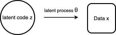
Suppose we have data $x$ and hypothesize data is generated by a latent process $\theta$ , starting from a latent code $z$ .

Then what we want to do is to maximize $\log p_\theta(x)$ , sometimes called the “log evidence”. Let $p_\theta(z|x)$ to describe the posterior probability of $z$ given observing $x$ and $p_\theta(x,z)$ to describe the joint probability of $x$ and $z$ . Note that, $p_\theta(z|x)$ is infeasible to compute in general. Therefore, we introduce $q_\phi(z|x)$ to approximate $p_\theta(z|x)$ , with $\phi$ being learnable parameters. $q_\phi(z|x)$ is tractable, for example, a neural network with outputs representing a Gaussian distribution’s mean and variance but can only approximate the true posterior distribution, $p_\theta(z|x)$ . It turns out that $log p_\theta(x)$ can be rewritten into [see 6, page 22-23 for derivation]:
$log p_\theta = KL\left(q_\phi(z|x) \Vert p_\theta(z|x)\right) - KL\left(q_\phi(z|x) \Vert p_\theta(x, z) \right)$ .

We call the second term, $- KL\left(q_\phi(z|x) \Vert p_\theta(x, z)\right)$ , the evidence lower bound (ELBO). We have $log p_\theta \geq - KL\left(q_\phi(z|x) \Vert p_\theta(x, z)\right) = ELBO$ because $KL\left(q_\phi(z|x) \Vert p_\theta(z|x)\right) \geq 0$ . Therefore, we can maximize ELBO w.r.t. $\phi$ in order to maximize $log p_\theta(x)$ .

ELBO can be further derived into [see derivation in 5]:
$log p_\theta(x) \geq - KL\left(q_\phi(z|x) \Vert p_\theta(x, z)\right) = \newline \mathbb{E}_{z\sim q_\phi(z|x)}\left[ log p_\theta(x|z)\right] - KL\left( q_\phi(z|x) \Vert p(z) \right)$ ,
where $p(z)$ is the prior for the latent code (e.g., standard normal distributions). In VAE, we also use a deterministic neural network to approximate $log \; p_\theta(x|z) \approx log \; q_{\phi'}(x|z)$ . Overall, $\mathbb{E}_{z\sim q_\phi(z|x)}\left[ log q_{\phi'}(x|z)\right] - KL\left( q_\phi(z|x) \Vert p(z) \right)$ can be learned by minibatch samples and when ELBO is maximized, $q_\phi(z|x)$ infinitely approximates $p_\theta(z|x)$ .

Deep Variational Information Bottleneck

If you view VAE as a clever idea to encode information of $x$ (data) in an unsupervised learning setting, Deep Variational Information Bottleneck [2] is an extended idea to encode latent information from $x$ (data) to $y$ (label) in a supervised learning setting. The objective is to encode $x$ into latent code $z$ with as little mutual information as possible, while making $z$ preserve as much as possible mutual information with $y$ :

After some derivation shown in [2], we can show that we can also instead maximize a lower bound (notations slightly different than [2] because I want it to be consistent in this post):
$I(z;y) - \beta I(z;x) \geq \mathbb{E}_{z\sim q_{\phi}(z|x)}\left[ log q_{\phi'}(y|z) \right]-\beta KL\left(q_\phi(z|x) \Vert p(z)\right),$
where, again, $q_\phi(z|x)$ is the variational distribution to the true posterior distribution $p_\theta(z|x)$ and $q_{\phi'}(y|z)$ is the decoder network.

Meta-RL Exploration By a Deep Variational Information Bottleneck Method

With all necessary ingredients introduced, we now introduce how Meta-RL exploration can benefit from Information Bottleneck [1]. The basic Meta-RL setup is that we have diverse environments. Each environment is represented with a tensor (could be a one-hot encoding) $\mu$ , which is known at training time but unknown at testing time. The authors of [1] propose to learn two policies: $\pi^{exp}_{\phi}(a|s)$ for exploring environments with the goal to collect as much information about the environment as possible, and $\pi^{task}_{\theta}(a|s, z)$ for exploiting an environment with a known encoded tensor $z$ . In training time, $z \sim \mathcal{F}_{\psi}(z|u)$ , an encoder to encode environment tensor $u$ (available in training time) or $z \sim q_\omega(z|\tau^{exp})$ , a variational encoder which converts the trajectory generated by $\pi^{exp}_{\phi}(a|s)$ to an encoded tensor. The variational encoder $q_\omega(z|\tau^{exp})$ will be learned to match $\mathcal{F}_{\psi}(z|u)$ in training time. Once $\theta$ , $\phi$ , $\omega$ , and $\psi$ are learned, at testing time, we can run $\pi^{exp}_{\phi}(a|s)$ to collect trajectories $\tau^{exp}$ , use $q_\omega(z|\tau^{exp})$ to determine the environment’s encoded tensor $z$ , and run $\pi^{task}_{\theta}(a|s, z)$ on top to maximize rewards.

The paper uses the mutual information / deep variational information bottleneck ideas in two places. First, when we learn $\pi^{task}_{\theta}(a|s, z)$ and $\mathcal{F}_{\psi}(z|u)$ , we use the following loss function to encourage $z$ encoding minimal information from $\mu$ :
$\text{minimize} \qquad I(z;u) \newline \text{subject to} \quad \mathbb{E}_{z \sim F_{\psi}(z|\mu)}\left[ V^{\pi_\theta^{task}}(z;\mu)\right]=V^*(\mu) \text{ for all } \mu$

The constrained optimization loss function can be converted to a unconstrained loss function by the lagrangian method, with $\lambda$ set as a hyperparameter [8]:
$\text{maximize}_{\psi, \theta}\quad \mathbb{E}_{\mu \sim p(\mu), z\sim F_{\psi}(z|\mu)}\left[V^{\pi_\theta^{task}}(z;\mu) \right] - \lambda I(z;\mu)$

Using the same derivation from [2] (Eqn. 13 & 14), we know the lower bound of $-I(z;u)$ is $-KL(F_{\psi}(z|\mu)\Vert p(z))$ , which has an analytic form when the prior $p(z)$ is chosen properly (e.g., Gaussian). Thus the unconstrained loss function can be maximized on a lower bound.

Second, we encourage to maximize the mutual information between the trajectories explored by $\pi^{exp}_{\phi}(a|s)$ and $z \sim F_{\psi}(z|\mu)$ :
$I(\tau^{exp};z) = H(z) - H(z|\tau^{exp}) \geq H(z) + \mathbb{E}_{\mu, z\sim F_\psi, \tau^{exp}\sim \pi^{exp}}\left[ q_\omega(z|\tau^{exp}) \right]$
(The inequality uses the fact that the KL divergence between the true posterior distribution and the variational distribution, $KL(p(z|\tau^{exp}) \Vert q_\omega(z|\tau^{exp}))$ , is greater than or equal to 0. )

As we see in the paper, $q_\omega$ is learned to match $\mathcal{F}_{\psi}(z|u)$ , while, with some trick to rearrange $\mathbb{E}_{\mu, z\sim F_\psi, \tau^{exp}\sim \pi^{exp}}\left[ q_\omega(z|\tau^{exp}) \right]$ , we can optimize $\pi^{exp}_{\phi}(a|s)$ in an MDP with reward set as information gain of each step.

References

[1] Decoupling Exploration and Exploitation for Meta-Reinforcement Learning
without Sacrifices: https://arxiv.org/pdf/2008.02790

[2] DEEP VARIATIONAL INFORMATION BOTTLENECK: https://arxiv.org/pdf/1612.00410

[3] https://en.wikipedia.org/wiki/Mutual_information

[4] https://czxttkl.com/2019/05/04/stochastic-variational-inference/

[5] https://czxttkl.com/2020/04/06/optimization-with-discrete-random-variables/

[6] https://www.cs.cmu.edu/~bhiksha/courses/deeplearning/Fall.2015/slides/lec12.vae.pdf

[7] https://stats.stackexchange.com/a/500240

[8] https://stats.stackexchange.com/questions/460984/are-lagrange-multipliers-of-regularization-terms-learned-or-set

View LLMs as compressors + Scaling laws

I feel it is a fascinating perspective to view LLMs as compressors. Today, we are going to introduce the basic idea of it.

We first use very layman terms to introduce what compression does. Compression can be seen as representing a stream of bits with a shorter stream of bits. It is based on assumption that there are certain repetitive patterns in the original stream so that we can represent those repetitive patterns with shorter codes. For example, if the original bit stream is “00001 00011 00001 00011…”, we can create a codebook, where “00001” is represented as “0” and “00011” is represented as “1”. Then, we can just use “010101…” plus the created codebook to represent the original bit stream. Anyone receiving the coded stream can uncover the original bit stream as long as they also receive the codebook.

There exist many compression algorithms. One algorithm is called arithmetic coding. It represents a bit stream by a float number between [0, 1] and its compressed stream will be the binary coding of that float number. Arithmetic coding can be easily connected to LLMs because when it compresses it utilizes $p(y|x_{<k})$ , which is exactly the next token prediction distribution.

We use the example in the paper [1] to illustrate how arithmetic coding works.

Suppose we have 3 tokens in the vocabulary (A, X, and I). To encode AIXI, we will look at the next-token prediction from a sequence predictor (LLM or any compression algorithm). Following Appendix A of [1], we have:

As we can see, we need to use 0101010 (7 bits) to represent AIXI. Other plausible sequences also need multiple bits to represent them. On average, the length of arithmetic code is larger than 1.

Now, let’s have a very hypothetical setting, where the LLM has more certain predictions. We have P(AIXI)=0.5 and P(AIXX)=0.5 and every other sequence has 0 sequence likelihood. In this case we only need to use 1 bit to represent the two plausible sequence. Therefore, we can conclude that if a LLM can predict sequences more accurately, it will compress data using shorter lengths of arithmetic codes.

References:

[1] Language Modeling Is Compression: https://arxiv.org/abs/2309.10668

[2] LLMZip: Lossless Text Compression using Large Language Models: https://arxiv.org/abs/2306.04050

[3] How Language Models Beat PNG and FLAC Compression & What It Means: https://blog.codingconfessions.com/p/language-modeling-is-compression

TQQQ/UPRO + volatility

In the past, we have tested TQQQ/UPRO on simulation data and real data. Today, I encountered an interesting video talking about using volatility indicators to decide when to hold leveraged ETFs. Here, I am just recording its link and its main result. We may come back and add more discussions in the future.

Update 2024-07-08

Personally, I don’t completely trust volatility indicators that much. I prefer staying in the market with a right re-balance strategy. I see a strategy online, which is about rebalancing between TQQQ and BTLA (an ETF aiming for stability) annually to weather extreme volatility. When backtesting on last 3~5 years, this strategy seems to outperform holding TQQQ alone. Here is more analysis.

I created 3 portfolios, where portfolio 1=holding TQQQ 100%, portfolio 2=holding 50% TQQQ and 50% BTLA, and portfolio 3=holding 70% TQQQ and 30% BTAL. We can see that portfolio 3 has similar performance with portfolio 1 while having about half volatility. Portfolio 2 is more stable but also less return overall.

However, portfolio 3 still has -47.32% worst year and -48.10% max drawdown. So next I am trying different ratios between TQQQ and BTLA. In the new comparison, portfolio 1= 70% TQQQ and 30% BTAL, portfolio 2=65% TQQQ and 35% BTAL, portfolio 3=60% TQQQ and 40% BTAL.

But we see that we have to trade stability with return. Personally, my comfortable ratio of TQQQ is between 65%~70% because the max drawdown is less than 50%, some threshold I can bare with.

I also find some alternative to BTAL because its return is too flat. I believe JEPI is a better option because it has monthly dividend to grow itself. hence much higher total return over long term. The largest drawdown of JEPI is about 1-125/140=10%, while that of BTAL is even higher 1-75/87=14%.

To conclude, I’ll stick to 65% TQQQ and 35% JEPI in the future to have a good return and stability balance.

The portfolio backtest tool I used is available at https://valueinvesting.io/backtest-portfolio

Update 2025-05-11:

I saw another post saying other good volatility indicators are moving average 200 and CNN Fear & Greedy Index: https://seekingalpha.com/article/4699905-tqqq-two-ways-to-tame-the-volatility-and-capture-far-more-upside

Update 2025-08-13:

In practice, the re-balance strategy or moving-average-200 strategy will be expensive in execution because of long-term/short-term capital gain tax. Personally, I would favor an approximate re-balance strategy in which we never sell stocks and only choose either of the two stocks to pour DCA money into. So I wrote a simple script to test this approximate rebalance strategy, with different target ratios between TQQQ:SPY.

</p>
# https://stockcharts.com/h-sc/ui
 
import yfinance as yf
 
TICK_RATIO = 0.5
 
def my_stock_return(tick):
    stock = yf.Ticker(tick)
    stock_hist = stock.history(start="2018-04-01", end="2025-08-13")

    spy = yf.Ticker("SPY")
    spy_hist = spy.history(start="2018-04-01", end="2025-08-13")

    days = 0
    total_tick_share = 0
    total_spy_share = 0
    single_invest = 3000
    total_invest = 0
    total_invest_time = 0
    total_tick_value = 0.01
    total_spy_value = 0.01

    max_value = 0
    max_drawback = 0

    for a, b in zip(stock_hist.iterrows(), spy_hist.iterrows()):
        idx, row = a
        _, spy_row = b

        if days % 10 != 0:
            days += 1
            continue
        
        total_invest += single_invest
        total_invest_time += 1
        if total_tick_value / (total_tick_value + total_spy_value) < TICK_RATIO:
            single_tick_share = single_invest / row['Open']
            total_tick_share += single_tick_share
        else:
            single_spy_share = single_invest / spy_row['Open']
            total_spy_share += single_spy_share
        total_tick_value = total_tick_share * row['Close']
        total_spy_value = total_spy_share * spy_row['Close']
        total_value = total_tick_value + total_spy_value

        if total_value > max_value:
            max_value = total_value
        drawback = (max_value - total_value) / max_value * 100
        if drawback > max_drawback:
            max_drawback = drawback
 
        days += 1
 
    total_tick_value = total_tick_share * stock_hist.iloc[-1]["Close"]
    total_spy_value = total_spy_share * spy_hist.iloc[-1]["Close"]
    total_value = total_tick_value + total_spy_value
 
    print(f"tick={tick}")
    print(f"days: {days}")
    print(f'last day close: {stock_hist.iloc[-1]["Close"]}')
    print(f"total_tick_share: {total_tick_share}")
    print(f"total_spy_share: {total_spy_share}")
    print(f'total_tick_value = total_share * last day close: {total_tick_value}')
    print(f'total_spy_value = total_share * last day close: {total_spy_value}')
    print(f"total_value = total_tick_value + total_spy_value: {total_value}")
    print(f"total_invest: {total_invest}, total_invest_time: {total_invest_time}")
    print(f"total gain: {(total_value / total_invest - 1) * 100}%")
    print(f"max drawback: {max_drawback}%")
 
 
my_stock_return("TQQQ")
print("\n")

<p>

Here is the result:

Period: 2018-04-01 ~ 2025-08-13
- TQQQ:SPY=0:100. Total gain: 80%, Max drawdown: 23%
- TQQQ:SPY=40:60. Total gain: 163%, Max drawdown: 45%
- TQQQ:SPY=50:50. Total gain: 178%, Max drawdown: 50%
- TQQQ:SPY=60:40. Total gain: 192%, Max drawdown: 54%
- TQQQ:SPY=70:30. Total gain: 208%, Max drawdown: 58%
- TQQQ:SPY=80:20. Total gain: 224%, Max drawdown: 64%
- TQQQ:SPY=100:0. Total gain: 257%, Max drawdown: 76%
- (Baesline) QLD:SPY=100:0. Total gain: 210%, Max drawdown: 55%
Period: 2015-04-01 ~ 2025-08-13
- TQQQ:SPY=0:100. Total gain: 125%, Max drawdown: 27%
- TQQQ:SPY=40:60. Total gain: 299%, Max drawdown: 54%
- TQQQ:SPY=50:50. Total gain:344%, Max drawdown: 60%
- TQQQ:SPY=60:40. Total gain: 395%, Max drawdown: 64%
- TQQQ:SPY=70:30. Total gain: 450%, Max drawdown: 68%
- TQQQ:SPY=80:20. Total gain: 509%, Max drawdown: 71%
- TQQQ:SPY=100:0. Total gain: 662%, Max drawdown: 79%
- (Baesline) QLD:SPY=100:0. Total gain: 457%, Max drawdown: 58%

Note that, if you have accumulated so much total value and your DCA money becomes so little relative to the total value, then this approximate rebalance strategy will be essentially the same as not rebalancing. So some manual rebalancing (and consequently some tax occurred) is still necessary at that point. Ultimately, when you have accumulated so much total value, I expect we should still rely on annually/semi-annually manual rebalancing as described in 2024-07-08 update. If you look at our baseline, which purely invested in QLD (2x leveraged QQQ), you can find it can achieve better gain with similar drawdown as the corresponding TQQQ:SPY ratio. This again illustrates that the approximate rebalance strategy I am implementing here is not optimal.

I am relying on https://valueinvesting.io/backtest-portfolio to re-test the semi-annually rebalancing strategy.

From Jan 2013 – July 2025, initial money is 10K, then invest 5K every month (inflation adjusted), rebalance semi-annually
100% TQQQ. Final balance: 11M, max drawdown: 78%
TQQQ:SPY=80:20. Final balance: 10.6M, max drawdown: 66%
TQQQ:SPY=70:30. Final balance: 9.6M, max drawdown: 60%
TQQQ:SPY=60:40. Final balance: 8.3M, max drawdown: 54%
TQQQ:SPY=50:50. Final balance: 7M, max drawdown: 49%
100% QLD. Final balance: 7M, max drawdown: 59%

This time, we can see that the real rebalance strategy (TQQQ:SPY=60:40) can outperform buying 100% QLD with similar max drawdown.

On the other hand, we could apply any re-balance or moving-average-200 strategy without worrying about tax in tax-advantaged accounts like 401k. I take an additional investigation on how good the moving-average-200 strategy is (i.e., sell all TQQQ shares if Nasdaq index is below MA200 and only buy TQQQ if Nasdaq index is above MA200). The result is this strategy will reduce max drawdown while keeping he same net profit. But this strategy seems only overfitted to TQQQ – if I test on UPRO, this strategy is far worse.

More details in DPO

In this post, we dig into more details of Direct Preference Optimization [1], a popular method used in RLHF.

First, we start from the normal RLHF objective that is typically used in PPO literature, which is equation 3 in the DPO paper [1]. Typically, we have input prompts $x$ and an LLM’s responses $y$ . The objective of optimizing the LLM, $\pi_\theta$ , is:

$\max_{\pi_\theta} \mathbb{E}_{x \sim \mathcal{D}, y\sim \pi_\theta(y|x)}[r_\phi(x,y)] - \beta \mathbb{D}_{KL}[\pi_\theta(y|x) || \pi_{ref}(y|x)],$
which states that we want to maximize the reward model score $r_\phi(x,y)$ but also, in balance, to minimize the KL-divergence from a reference policy $\pi_{ref}(y|x)$ .

The equation above can be rewritten by incorporating the KL-divergence term into the reward function. Because $\mathbb{D}_{KL}[\pi_\theta(y|x) || \pi_{ref}(y|x)]=\sum_y \pi_\theta(y|x) \log\frac{\pi_\theta(y|x)}{\pi_{ref}(y|x)} =\mathbb{E}_{y\sim \pi_\theta(y|x)}[\log\frac{\pi_\theta(y|x)}{\pi_{ref}(y|x)}]$ , we have

$\max_{\pi_\theta} \mathbb{E}_{x \sim \mathcal{D}, y\sim \pi_\theta(y|x)}\left[r_\phi(x,y) - \beta (\log \pi_\theta(y|x) - \log \pi_{ref}(y|x)) \right] \newline = \mathbb{E}_{x \sim \mathcal{D}, y\sim \pi_\theta(y|x)}\left[r_\phi(x,y) + \beta \log \pi_{ref}(y|x) - \beta \log \pi_\theta(y|x) \right] \newline \text{because }-\log \pi_\theta(y|x) \text{ is an unbiased estimator of entropy } \mathcal{H}(\pi_\theta)=-\sum_y \pi_\theta(y|x) \log \pi_\theta(y|x), \newline \text{we can transform to equation 2 in [3]} \newline= \mathbb{E}_{x \sim \mathcal{D}, y\sim \pi_\theta(y|x)}\left[r_\phi(x,y) + \beta \log \pi_{ref}(y|x) + \beta \mathcal{H}(\pi_\theta)\right]$

Now there are two perspectives for how to solve the maximization problem above. The first solution is based on the DPO paper’s Appendix A.1 [1]:

$\max_{\pi_\theta} \mathbb{E}_{x \sim \mathcal{D}, y\sim \pi_\theta(y|x)}\left[r_\phi(x,y) - \beta (\log \pi_\theta(y|x) - \log \pi_{ref}(y|x)) \right] \newline = \min_{\pi_\theta} \mathbb{E}_{x \sim \mathcal{D}, y\sim \pi_\theta(y|x)} \left[ \log \frac{\pi_\theta(y|x)}{\pi_{ref}(y|x)} - \frac{1}{\beta}r_\phi(x,y) \right] \newline =\min_{\pi_\theta} \mathbb{E}_{x \sim \mathcal{D}, y\sim \pi_\theta(y|x)} \left[ \log \frac{\pi_\theta(y|x)}{\pi_{ref}(y|x)} - \log exp\left(\frac{1}{\beta}r_\phi(x,y)\right) \right] \newline = \min_{\pi_\theta} \mathbb{E}_{x \sim \mathcal{D}, y\sim \pi_\theta(y|x)} \left[ \log \frac{\pi_\theta(y|x)}{\pi_{ref}(y|x)exp\left(\frac{1}{\beta}r_\phi(x,y)\right)} \right] \newline \pi_{ref}(y|x)exp\left(\frac{1}{\beta}r_\phi(x,y)\right) \text{ may not be a valid distribution. But we can define a valid distribution:} \pi^*(y|x)=\frac{1}{Z(x)}\pi_{ref}(y|x)exp\left(\frac{1}{\beta}r_\phi(x,y)\right), \text{ where } Z(x) \text{ is a partition function not depending on } y \newline = \min_{\pi_\theta} \mathbb{E}_{x \sim \mathcal{D}, y\sim \pi_\theta(y|x)} \left[ \log \frac{\pi_\theta(y|x)}{\pi^*(y|x)} \right]$
Due to the so-called Gibbs’ inequality, the optimal solution is when $\pi^*_\theta(y|x) = \pi^*(y|x)=\frac{1}{Z(x)}\pi_{ref}(y|x)exp\left(\frac{1}{\beta}r_\phi(x,y)\right)$ everywhere.

The second solution is based on Maximum Entropy RL [6] and can be solved by the method of Lagrangian multipliers. The constrained objective function from what we derived above is:

$\max_{\pi_\theta} \mathbb{E}_{x \sim \mathcal{D}, y\sim \pi_\theta(y|x)}\left[\underbrace{r_\phi(x,y) + \beta \log \pi_{ref}(y|x)}_{\text{actual reward function}} + \beta \mathcal{H}(\pi_\theta)\right] \newline s.t. \quad \sum\limits_y \pi_\theta(y|x)=1,$

which is exactly the objective function of MaxEnt RL with the actual reward as $r(x,y)=r_\phi(x,y) + \beta \log \pi_{ref}(y|x)$ . Note, we are solving a one-step MaxEnt RL problem. So we can use the Lagrangian multipliers method to reach the same solution. See 1hr:09min in [5] for more details.

Now we have introduced two ways to derive the optimal solution of $\pi^*_\theta(y|x) = \frac{1}{Z(x)}\pi_{ref}(y|x)exp\left(\frac{1}{\beta}r_\phi(x,y)\right)$ . With some arrangement, we can see that this formula entails that the reward function can be represented as a function of $\pi^*_\theta(y|x)$ and $\pi_{ref}(y|x)$ :

$r_\phi(x,y)=\beta \log \pi^*_\theta(y|x) - \beta \log \pi_{ref} (y|x) - Z(x)$

With collected human preference data $(x, y_w, y_l) \sim \mathcal{D}$ and a Bradley-Terry model, we know that
$p(y_w > y_l | x) = \frac{exp(r(x, y_w))}{exp(r(x, y_w)) + exp(r(x, y_l))}$

We can convert $p(y_w > y_l | x)$ into the logit [7]:
$logit (y_w > y_l | x) = log \frac{p(y_w > y_l | x) }{1 - p(y_w > y_l | x) } = r(x, y_w) -r(x, y_l),$
which can be solved by maximum likelihood as in logistic regression:
$-\mathbb{E}_{(x, y_w, y_l) \sim \mathcal{D}}\left[\log \sigma \left(r(x, y_w) - r(x, y_l)\right) \right] \newline = -\mathbb{E}_{(x, y_w, y_l) \sim \mathcal{D}}\left[ \log \sigma \left( \left(\beta \log \pi^*_\theta(y_w|x) - \beta \log \pi_{ref} (y_w | x) \right) - \left( \beta \log \pi^*_\theta(y_l |x) - \beta \log \pi_{ref} (y_l | x) \right)\right)\right] \newline = -\mathbb{E}_{(x, y_w, y_l) \sim \mathcal{D}}\left[ \log \sigma \left( \beta \log \frac{\pi^*_\theta(y_w|x)}{\pi_{ref} (y_w | x)} - \beta \log \frac{\pi^*_\theta(y_l |x)}{\pi_{ref} (y_l | x)} \right) \right]$

We have been deriving the optimal DPO solution assuming the environment is a one-step MDP (i.e., bandits) because we only receive a reward for an entire response. However, if we have dense rewards on each token, the decoding process is essentially a token-level MDP, where decoding each token is one step in the MDP. The Bradley-Terry model in the token-level MDP becomes:
$p(y_w > y_l | x) = \frac{exp \left(\sum_{i=1}^N r(x, y_{w^, <i}, y^i_w) \right)}{exp \left( \sum_{i=1}^N r(x, y_{w, <i}, y^i_w)\right) + exp \left( \sum_{i=1}^M r(x, y_{l, <i}, y^i_l) \right)}$

In such a case, does the DPO loss function, $-\mathbb{E}_{(x, y_w, y_l) \sim \mathcal{D}}\left[ \log \sigma \left( \beta \log \frac{\pi^*_\theta(y_w|x)}{\pi_{ref} (y_w | x)} - \beta \log \frac{\pi^*_\theta(y_l |x)}{\pi_{ref} (y_l | x)} \right) \right]$ , still align the underlying policy to the Bradley-Terry preference probability defined in the token-level MDP? The answer is yes as proved in [3]. We first need to make an interesting connection between the decoding process and multi-step Maximum Entropy RL. (Note, earlier in this post, we have made a connection between on-step Maximum Entropy RL and DPO in the setting of bandits.)

In multi-step Maximum Entropy RL [6], the objective is $\pi^*_{MaxEnt} = \arg\max_\pi \sum_t \mathbb{E}_{(s_t, a_t) \sim \pho_\pi} \left[ r(s_t, a_t) + \beta \mathcal{H}\left(\pi(\cdot | s_t)\right)\right]$ . People have proved the optimal policy can be derived as $\pi^*_{MaxEnt}(a_t|s_t) = \exp \left( \frac{1}{\beta} \left( Q^*_{soft}(s_t, a_t) - V^*_{soft}(s_t) \right)\right),$ where $Q^*_{soft}(s_t, a_t)$ and $V^*_{soft}(s_t)$ are the corresponding Q-function and V-function in the MaxEnt RL [8]. For any LLM, its decoding policy $\pi_\theta(y_i|x, y_{<i})$ is a softmax over the whole vocabulary. Therefore, $\pi_\theta(y_i|x, y_{<i})$ can be seen as an optimal policy of a MaxEnt RL in a token-level MDP with a particular reward function (however the reward function is unknown to us).

Based on the definition of Q functions and V functions (with a discount factor equal to 1), we have $Q^*_{soft}(x, y_{<i}, y^i) = r(x, y_{<i}, y^i) + \beta \log \pi_{ref}(y_i|x, y_{<i}) + V^*_{soft}(x, y_{<i})$ in terms of an LLM’s decoding process. We could re-arrange the formula to represent per-token reward as:
$r(x, y_{<i}, y^i) \newline= Q^*_{soft}(x, y_{<i}, y^i) - \beta \log \pi_{ref}(y_i|x, y_{<i}) - V^*_{soft}(x, y_{<i}) \newline =\left(Q^*_{soft}(x, y_{<i}, y^i) - V^*_{soft}(x, y_{<i})\right) - \beta \log \pi_{ref}(y_i|x, y_{<i}) \newline \qquad = \beta \log \pi^*(y_i|x, y_{<i}) - \beta \log \pi_{ref}(y_i|x, y_{<i})$

The logit of the Bradley-Terry model under the token-level MDP is then:
$logit (y_w > y_l | x) \newline = \sum\limits^N_{i=1}r(x, y_{w, <i}, y_w^i) - \sum\limits^M_{i=1}r(x, y_{l, <i}, y_l^i) \newline = \beta \sum\limits_{i=1}^{N}\log \frac{\pi_\theta(y_w^i | x, y_{w, <i})}{\pi_{ref}(y_w^i | x, y_{w,<i})} - \beta \sum\limits_{i=1}^M \log \frac{\pi_\theta(y_l^i | x, y_{l, <i})}{\pi_{ref}(y_l^i | x, y_{l,<i})}$

By learning this logit using maximum likelihood, we reach the same loss function as we derive in the bandits setting:
$-\mathbb{E}_{(x, y_w, y_l) \sim \mathcal{D}} \left[ \log \sigma \left(\beta \sum\limits_{i=1}^{N}\log \frac{\pi_\theta(y_w^i | x, y_{w, <i})}{\pi_{ref}(y_w^i | x, y_{w,<i})} - \beta \sum\limits_{i=1}^M \log \frac{\pi_\theta(y_l^i | x, y_{l, <i})}{\pi_{ref}(y_l^i | x, y_{l,<i})} \right) \right] \newline = -\mathbb{E}_{(x, y_w, y_l) \sim \mathcal{D}}\left[ \log \sigma \left( \beta \log \frac{\pi^*_\theta(y_w|x)}{\pi_{ref} (y_w | x)} - \beta \log \frac{\pi^*_\theta(y_l |x)}{\pi_{ref} (y_l | x)} \right) \right]$

A few notes to conclude this post:

Adding a KL divergence penalty in tandem with reward model scores seems to be just one option of telling the LLM to not deviate much from the reference policy. In theory, there could be other regularizers (e.g., L2 norm). But, surprisingly, using KL divergence penalty makes very interesting connection to Maximum Entropy RL and thus provides many theoretical groundings for DPO.
In practice, our preference data is collected once in advance using a mix of previous policies. In other words, preference data does not come from the LLM policy being updated. So in practice DPO is in fact an off-policy algorithm and data efficiency may not be optimal. (Note, if we have infinite diverse preference data not coming from the incumbent DPO policy, DPO may still converge to the optimal policy, just that the data efficiency is not optimal.) People have since proposed methods to generate more on-policy preference data: [9, 10, 11]

Reference

Direct Preference Optimization: Your Language Model is Secretly a Reward Model: https://arxiv.org/abs/2305.18290
Reinfocement Learning in LLMs: https://czxttkl.com/2024/01/23/reinfocement-learning-in-llms/
From r to Q∗: Your Language Model is Secretly a Q-Function: https://arxiv.org/abs/2404.12358
Controlled decoding from language models: https://arxiv.org/abs/2310.17022
L1 MDPs, Exact Solution Methods, Max-ent RL (Foundations of Deep RL Series): https://www.youtube.com/watch?v=2GwBez0D20A
Reinforcement Learning with Deep Energy-Based Policies: https://arxiv.org/pdf/1702.08165
https://en.wikipedia.org/wiki/Bradley%E2%80%93Terry_model#Definition
http://www.lamda.nju.edu.cn/yanggy/slide/Maximum_entropy_RL_Guoyu_Yang.pdf
Direct Language Model Alignment from Online AI Feedback: https://arxiv.org/abs/2402.04792
Statistical Rejection Sampling Improves Preference Optimization: https://arxiv.org/abs/2309.06657
Some things are more CRINGE than others: Iterative Preference Optimization with the Pairwise Cringe Loss: https://arxiv.org/abs/2312.16682

Minimal examples of HuggingFace LLM training

I’m sharing a minimal example of training an LLM model using HuggingFace’s libraries trl/transformers/evaluate/datasets/etc. The example is mainly borrowed from https://wandb.ai/capecape/alpaca_ft/reports/How-to-Fine-tune-an-LLM-Part-3-The-HuggingFace-Trainer–Vmlldzo1OTEyNjMy and its github repo https://github.com/tcapelle/llm_recipes/blob/main/scripts/train_hf.py.

Here is the full file:

import wandb
from datasets import load_dataset

# if you can't find libwebp library, use brew update && brew install webp
import evaluate
import numpy as np
import torch
from transformers import TrainingArguments
from trl import SFTTrainer
from transformers import (
    AutoModelForCausalLM, AutoTokenizer, AutoConfig,
    LlamaConfig, LlamaModel,
)
from transformers import GenerationConfig
from transformers.integrations import WandbCallback
from tqdm import tqdm


def token_accuracy(eval_preds):
    token_acc_module = evaluate.load("accuracy")
    logits, labels = eval_preds
    # shape: batch_size x max_sequence_length
    predictions = np.argmax(logits, axis=-1)
    # accuracy only accepts 1d array. So if the batch contains > 1 datapoints,
    # the accuracy is based on flattened arrays
    # https://huggingface.co/spaces/evaluate-metric/accuracy
    return token_acc_module.compute(
        predictions=predictions.flatten().astype(np.int32),
        references=labels.flatten().astype(np.int32),
    )


def prompt_no_input(row):
    return ("Below is an instruction that describes a task. "
            "Write a response that appropriately completes the request.\n\n"
            "### Instruction:\n{instruction}\n\n### Response:\n{"
            "output}").format_map(
        row
    )


def prompt_input(row):
    return (
        "Below is an instruction that describes a task, paired with an input "
        "that provides further context. "
        "Write a response that appropriately completes the request.\n\n"
        "### Instruction:\n{instruction}\n\n### Input:\n{input}\n\n### "
        "Response:\n{output}").format_map(
        row
    )


def create_alpaca_prompt(row):
    return prompt_no_input(row) if row["input"] == "" else prompt_input(row)


class LLMSampleCB(WandbCallback):
    def __init__(
            self, trainer, test_dataset, num_samples=10, max_new_tokens=256,
            log_model="checkpoint"
    ):
        super().__init__()
        self._log_model = log_model

        def create_prompt_no_anwer(row):
            row["output"] = ""
            return {"text": create_alpaca_prompt(row)}

        self.sample_dataset = test_dataset.select(range(num_samples)).map(
            create_prompt_no_anwer
        )
        self.model, self.tokenizer = trainer.model, trainer.tokenizer
        self.gen_config = GenerationConfig.from_pretrained(
            trainer.model.name_or_path,
            max_new_tokens=max_new_tokens
        )

    def generate(self, prompt):
        tokenized_prompt = self.tokenizer(prompt, return_tensors='pt')[
            'input_ids']
        with torch.inference_mode():
            output = self.model.generate(
                inputs=tokenized_prompt, generation_config=self.gen_config
            )
        return self.tokenizer.decode(
            output[0][len(tokenized_prompt[0]):], skip_special_tokens=True
        )

    def samples_table(self, examples):
        records_table = wandb.Table(
            columns=["prompt", "generation"] + list(
                self.gen_config.to_dict().keys()
            )
        )
        for example in tqdm(examples):
            prompt = example["text"]
            generation = self.generate(prompt=prompt)
            records_table.add_data(
                prompt, generation, *list(self.gen_config.to_dict().values())
            )
        return records_table

    def on_evaluate(self, args, state, control, **kwargs):
        super().on_evaluate(args, state, control, **kwargs)
        records_table = self.samples_table(self.sample_dataset)
        self._wandb.log({"sample_predictions": records_table})
        print("log once")


def param_count(m):
    params = sum([p.numel() for p in m.parameters()]) / 1_000_000
    trainable_params = sum(
        [p.numel() for p in m.parameters() if p.requires_grad]
    ) / 1_000_000
    print(f"Total params: {params:.2f}M, Trainable: {trainable_params:.2f}M")
    return params, trainable_params


def trl_train():
    wandb.login(key='replace_with_your_own')

    lr = 2e-5
    batch_size = 8
    max_steps = 4
    # evaluate every eval_steps. so if we set max_steps = 4 and
    # eval_steps = 2, we will evaluate twice during training
    eval_steps = 2
    num_eval_data = 5
    num_wandb_cb_eval_data = 7
    wandb_cb_max_new_tokens = 256
    num_train_epochs = 1
    max_seq_length = 1024
    gradient_accumulation_steps = 1
    gradient_checkpointing = False
    output_dir = "./output/"

    run = wandb.init(
        project="second_project",
        config={
            "lr": lr,
            "batch_size": batch_size,
            "max_steps": max_steps,
            "eval_steps": eval_steps,
            "num_eval_data": num_eval_data,
            "num_wandb_cb_eval_data": num_wandb_cb_eval_data,
        },
    )

    alpaca_ds = load_dataset("winglian/alpaca-gpt4-split")

    train_dataset = alpaca_ds["train"]
    eval_dataset = alpaca_ds["test"]

    model_id = 'meta-llama/Llama-2-7b-hf'
    # try different ways to initialize a llama model
    # method 1: construct LLamaModel from LlamaConfig
    # https://huggingface.co/docs/transformers/v4.37.2/en/model_doc
    # /llama2#transformers.LlamaConfig
    # configuration = LlamaConfig(
    #     num_hidden_layers=2,
    #     hidden_size=32,
    #     intermediate_size=2,
    #     num_attention_heads=1,
    #     num_key_value_heads=1,
    # )
    # model = LlamaModel(configuration)
    # param_count(model)

    # method 2 & 3 need to wait for token approval
    # https://huggingface.co/meta-llama/Llama-2-7b-hf
    # method 2: load config first, tune down model size, then initialize the actual LLM
    # https://discuss.huggingface.co/t/can-i-pretrain-llama-from
    # -scratch/37821/8
    config = AutoConfig.from_pretrained(model_id)
    config.num_hidden_layers = 1
    config.hidden_size = 2
    config.intermediate_size = 2
    config.num_attention_heads = 1
    config.num_key_value_heads = 1
    model = AutoModelForCausalLM.from_config(config)
    param_count(model)

    # method 3: directly load pretrained llama model, which may encounter OOM
    # on a consumer cpu machine
    # model = AutoModelForCausalLM.from_pretrained(
    #     model_id,
    #     device_map="auto",
    #     trust_remote_code=True,
    #     low_cpu_mem_usage=True,
    #     torch_dtype=torch.bfloat16,
    #     load_in_8bit=True,
    # )

    training_args = TrainingArguments(
        output_dir=output_dir,
        use_cpu=True,
        report_to="wandb",
        per_device_train_batch_size=batch_size,
        bf16=True,
        learning_rate=lr,
        lr_scheduler_type="cosine",
        warmup_ratio=0.1,
        max_steps=max_steps,
        eval_steps=eval_steps,
        num_train_epochs=num_train_epochs,
        gradient_accumulation_steps=gradient_accumulation_steps,
        gradient_checkpointing=gradient_checkpointing,
        gradient_checkpointing_kwargs={"use_reentrant": False},
        evaluation_strategy="steps",
        # logging strategies
        logging_strategy="steps",
        logging_steps=1,
        save_strategy="no",
    )
    tokenizer = AutoTokenizer.from_pretrained(model_id)
    tokenizer.pad_token = tokenizer.eos_token

    trainer = SFTTrainer(
        model,
        tokenizer=tokenizer,
        args=training_args,
        train_dataset=train_dataset,
        eval_dataset=eval_dataset.select(list(range(num_eval_data))),
        # this tells the trainer to pack sequences of `max_seq_length`
        # see illustration in https://wandb.ai/capecape/alpaca_ft/reports/How
        # -to-Fine-tune-an-LLM-Part-3-The-HuggingFace-Trainer--Vmlldzo1OTEyNjMy
        packing=True,
        max_seq_length=max_seq_length,
        formatting_func=create_alpaca_prompt,
        compute_metrics=token_accuracy,  # only call at evaluation
    )
    wandb_callback = LLMSampleCB(
        trainer, eval_dataset,
        num_samples=num_wandb_cb_eval_data,
        max_new_tokens=wandb_cb_max_new_tokens,
    )
    trainer.add_callback(wandb_callback)
    trainer.train()
    wandb.finish()

    # other materials:
    # fine tune ppo vs dpo
    # trl stackllama tutorial:
    # https://huggingface.co/docs/trl/using_llama_models
    # trl readme: https://github.com/huggingface/trl/tree/main?tab=readme-ov
    # dpo - trl: https://huggingface.co/blog/dpo-trl


if __name__ == '__main__':
    trl_train()

Now let’s examine the code in more details:

First, we initialize a weights & bias project (wandb.init(...)), which is used for logging intermediate training/evaluation results. It is a very convenient tool for logging and visualization.

Then, we use load_dataset(...) , an api from HuggingFace’s dataset library, to load a specific data. HuggingFace hosts many awesome datasets at https://huggingface.co/datasets.

Next, we initialize an actual LLM. Since this is a minimal example, I created a tiny LLM by modifying its config to have very few hidden layers and hidden sizes.

Next, we initialize TrainingArguments. We may need to be familiar with several concepts in TrainingArguments, such as gradient accumulation.

We then initialize a tokenizer, which is trivial by calling HuggingFace’s API AutoTokenizer.from_pretrained(...).

We then initialize SFTTrainer, the main class for training and evaluating the LLM. Setting packing=True means that we pack multiple individual sequences into a fixed-length sequence so that we can avoid much padding. Individual sequences are usually separated with an eos token.

We also initialize a callback, which is called only in the evaluation stage. The callback class needs to first remove output in the dataset for evaluation.

We now look at the results logged in wandb (example https://wandb.ai/czxttkl/third_project/runs/hinck0h5):

Since we specify max_steps=4 and eval_steps=2, we have 2 evaluations. The evaluation loss curves verifie we indeed log 2 evaluation results.
we have a table showing the results from the callback. We can verify that prompts indeed have outputs removed. We can also use runs.history.concat["sample_predictions"] instead of runs.summary["sample_predictions"] to check the evaluation results from all evaluation runs (exactly 2 runs) (see the reference in https://wandb.ai/morg/append-to-table/reports/Append-to-Table–Vmlldzo0MjY0MDIx)

Causal Inference 102

In my blog, I have covered several pieces of information about causal inference:

Causal Inference: we talked about (a) two-stage regression for estimating the causal effect between X and Y even when there is a confounder between them; (b) causal invariant prediction
Tools needed to build an RL debugging tool: we talked about 3 main methods for causal relationship discovery – (a) noise model; (b) quantile regression with the idea of Kolmogorov complexity; (c) matching
Causal Inference in Recommendation Systems: we talked about backdoor/frontdoor adjustment and causal relationship discovery in a sequence modeling setting

This time, I read a paper about learning causal relationship from pure observational data [1]. It has a very clear introduction of causal inference, which inspires me to write another introduction post of causal inference.

Let’s start from basic definitions. Structural causal models (SCM), structural equation models (SEM), or functional causal models (FCM) all refer to the same thing: a graph which indicates causal relationships between nodes and causal relationships are encoded by functions and noises. [1] uses the notation of FCM primarily. Here is an example of an FCM:

collider definition [5]: if a node has two edges pointing to it, it is called a collider. In the example above, x5 is a collider. X3, X4, and X5 form the so-called “v-structure”.

d-separation definition: d-separation is used to determine if a node set X is independent of a node set Y, given a node set Z. Specifically, if X and Y are d-connected, then X and Y are dependent given Z, denoted as $X \not\!\perp\!\!\!\perp_G Y | Z$ ; if X and Y are d-separated, then X and Y are independent given Z, denoted as $X \perp\!\!\!\perp_G Y | Z$ . If two nodes are not d-connected, then they are d-separated. There are several rules for determining whether two nodes are d-connected or d-separated [3]. An interesting (and often non-intuitive) example is that in a v-structure like (X3, X4, X5) above: X3 is d-connected (i.e., dependent) to X4 given X5 (i.e., the collider), even though X3 and X4 has no direct edge in between [4].

Identifiability definition: An observational distribution of all variables could be resulted by different FCMs. Thus, we are not guaranteed to infer the correct causal relationship from observational data. That’s why FCM is a richer structure than pure observational data and using pure probabilistic distributions are not enough to do causal inference! Proposition 4.1 (non-uniqueness of graph structures) in [6] says that there will always be some graph structure to explain an observational data of two variables thus we can never determine the correct causal relationship without additional assumption. If, with correct assumptions, we can identify the ground truth FCM from observational data, we call the FCM is identifiable.

Faithfulness definition: We are given observational data and a hypothesized FCM. Running conditional independence tests on the observational distribution will give us all conditional independence relationships. If all the identified conditional independence relationships from the data are also entailed by the FCM, then the observational distribution is faithful to the FCM. Here is an example [7] that an observational distribution is unfaithful to an FCM:

In the FCM, we can see that A and D are d-connected, meaning A and D are dependent (given an empty set Z).
If A, B, C, and D have the linear relationships indicated as on the right, then $D=(\alpha\beta + \gamma\delta)A$ . When $\alpha\beta =- \gamma\delta$ , the conditional independence test will return us $\perp\!\!\!\perp$ . Therefore, the identified conditional independence relationship from the data is not entailed by the FCM.

In practice, inferring FCMs from observational data are based on the Causal Sufficiency Assumption (CSA), Causal Markov Assumption (CMA), and Causal Faithfulness Assumption (CFA) (more details in [1]). Based on these assumptions, inferring FCMs from observational data limits the space of plausible FCMs and involves the following steps:

Determine all possible causal relationships using conditional independent tests and derive the Completed Partially Directed Acyclic Graph (CPDAG)
For undeterminable causal relationships, use constraint-based methods, score-based methods, or hybrid methods to get the best hypothesis

Recall that based on non-uniqueness of graph structures, there will always be some graph structure to explain an observational data of two variables thus we can never determine the correct causal relationship without additional assumption. Now let’s look at what additional assumption we could have to facilitate causal discovery in real world:

LinGAM assumes a linear structure FCM with all variables are continuous:
$X_i = \sum\limits_k \alpha_k P_a^k(X_i)+E_i, \;\; i \in [1, N]$
The LinGAM paper proves that when all probability distributions of source nodes in the causal graph are non-Gaussian, FCM is fully identifiable.
The additive noise model (ANM) assumes that we can learn the true causal direction between X and Y when:
1. $Y=f(X)+E$
2. $f(\cdot)$ is not a linear model with Gaussian input and Gaussian noise
3. Only two variables are involved in the FCM (hence ANM is a bivariate method)
The causal additive model (CAM) is the counterpart of ANM when there are more than 2 variables. Its assumption is similar to ANM that $f(\cdot)$ cannot be a linear model with Gaussian input and Gaussian noise for the FCM to be identifiable. (I am not totally sure about CAM’s assumption. We may need to verify more carefully.)

Up to this point, we have finished the causal inference 102 introduction. The proposed method itself in [1] is interesting and useful to me because I need to conduct causal relationship discovery on observational data very often. And its neural network-based method seems general to handle practical data. There are many other causal relationship discovery methods. You can find more in an open source toolbox: [2]

References

[1] Learning Functional Causal Models with Generative Neural Networks: https://arxiv.org/abs/1709.05321

[2] https://fentechsolutions.github.io/CausalDiscoveryToolbox/html/causality.html

[3] https://yuyangyy.medium.com/understand-d-separation-471f9aada503

[4] https://stats.stackexchange.com/a/399010/80635

[5] https://en.wikipedia.org/wiki/Collider_(statistics)

[6] Elements of Causal Inference: https://library.oapen.org/bitstream/handle/20.500.12657/26040/11283.pdf?sequence=1&isAllowed=y

[7] https://www.youtube.com/watch?v=1_b7jgupoAE