Recent advances in Batch RL

I’ll introduce some recent papers advancing batch RL.

The first paper is Critic Regularized Regression [1]. It starts from a general form of actor-critic policy gradient objective function, where $Q_\theta$ is a learned critic function:

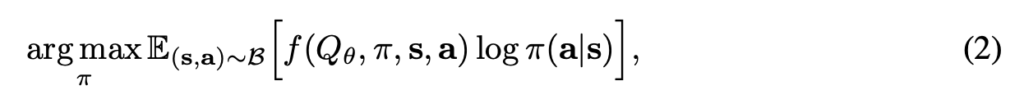
For a behavior cloning method, $f(Q_\theta, \pi, s, a) = Q_\theta(s, a)$ . However, we can do much more than that choice:

The CRR paper tested the first two choices, while another famous algorithm Advantage Weighted Behavior Model (ABM) from paper (Keep Doing What Worked: Behavioral Modelling Priors for Offline Reinforcement Learning) [2] used the third choice.

CRR can be connected to a popular family of policy gradient algorithms called Maximum a Posteriori Policy Optimisation (MPO) [3], which I think is better summarized in [2]. From [2], we can see that MPO solves problems in the following form:

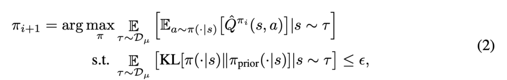
The optimal solution by MPO has a closed form expression: $\pi(a|s) \propto \pi_{prior}(a|s) exp(\hat{Q}^{\pi}(s,a) / \eta)$

In CRR, $\pi_{prior}$ is equal to the logging policy $\mu_\beta$ . So the optimal solution is supposed to be $\pi(a|s) \propto \mu_{\beta}(a|s) exp(\hat{Q}^{\pi}(s,a) / \eta)$ . The CRR paper points out it is equivalent to subtract the state value $V(s)$ from $\hat{Q}^{\pi}(s,a)$ , leading to $\pi(a|s) \propto exp(\hat{A}^{\pi}(s,a) / \eta)$ . (I am not sure how $\mu_{\beta}(a|s)$ is omitted. )

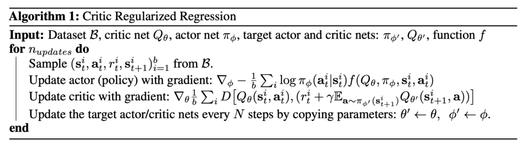
The overall learning loop of CRR is very straightforward:

Let’s look at how MPO is used in the ABM paper [2]. While $\pi_{prior}$ in CRR is the logging policy $\mu_\beta$ , $\pi_{prior}$ in ABM could also be a behavior cloning policy mimicking the logging policy or the advantaged-based behavior cloning policy.

As argued in [2], the reason to not simply using a behavior cloning prior is to avoid learning from a very mediocre logging policy: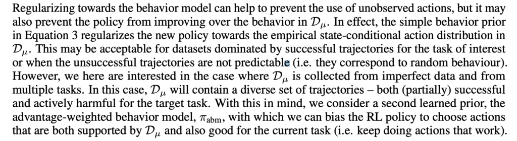

Once we obtain $\pi_{prior}$ , we can learn the RL policy $\pi$ using Eqn. 2. [2] provides two ways of optimization: (1) Expectation-Maximization, alternating between $\pi$ and the Lagrangian multiplier $\alpha$ ; (2) stochastic gradient descent with reparameterization trick because there is $\mathbb{E}_{a \sim \pi(\cdot|s)}$ in the objective.

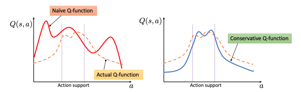
The next paper is conservative Q-learning [4]. The idea is simple though the proof in the paper is too dense to understand. I am following https://towardsdatascience.com/the-power-of-offline-reinforcement-learning-5e3d3942421c to illustrate its idea. In standard Q-learning, our loss function is:

$\begin{align*}\begin{split}L&=\mathbb{E}_{s,a\sim D}\left[\delta(s,a)\right]\\&=\mathbb{E}_{s,a\sim D} \left[ \left\| Q(s,a) - \left(r(s,a) + \gamma max_{a'}Q(s',a') \right) \right\|^2 \right] \end{split}\end{align*}$

A very conservative Q-learning loss function is:

$\begin{align*}\begin{split}L&=\mathbb{E}_{s,a\sim D}\left[\delta(s,a)\right] + \alpha \cdot \mathbb{E}_{s\sim D, a \sim \pi} \left[ Q(s,a)\right],\end{split}\end{align*}$

which can be understood intuitively as you are always dragging down the Q-values of whichever action selected by the learned policy.

However, the authors find in this way the Q values are learned too conservative. Therefore, they propose a relaxing version of loss:

$\begin{align*}\begin{split}L&=\mathbb{E}_{s,a\sim D}\left[\delta(s,a)\right] + \alpha \cdot \left( \mathbb{E}_{s\sim D, a \sim \pi} \left[ Q(s,a)\right] - \mathbb{E}_{s,a \sim D} \left[ Q(s,a)\right] \right),\end{split}\end{align*}$

This objective can be understood that we not only drag down the Q-values of the learned policy’s actions, but also pull up the Q-values of the logged actions. As a balance, the resultant Q-function is more conservative in actions not seen but less conservative in actions seen in the logged data.

Different batch RL can all be boiled down to how to extrapolate Q-values on unobserved/less observed (state, action) pairs. [5] provides a principled way to zero out those “uncertain” Q-values. Here are some basic notations for introducing their idea:

There are two paradigms of learning a policy from data: policy iteration and value iteration. [5]’s methodology can be plugged in either paradigm.

For policy iteration (they call MBS-PI):

For value iteration (they call MBS-QI):

You can see that their methods all come down a filter $\varepsilon$ , which simply zeros out Q values of (state, action) frequency less than a threshold:

It is interesting to see how we empirically compute $\hat{\mu}(s,a)$ , the count/probability distribution of encountering (state, action) pairs.

For discrete action problems, they discretize state spaces by binning each state feature dimension. Therefore, there are a finite number of (state, action) pairs for which they count frequencies.
For continuous action problems, we can train a VAE to learn $ELBO(s,a)$ , the lower bound of $\hat{\mu}(s,a)$ , as the objective function. Once the VAE is learned, we can compute $\varepsilon(s,a)$ by $\varepsilon(s,a) = \mathbb{I}(ELBO(s,a) > \text{thres})$ , where $\mathbb{I}(\cdot)$ is an indicator function.
For continuous action problems, another methodology, which is used in the paper, is to integrate with BCQ [7]. BCQ trains a conditional VAE to only sample actions similar to the data collection policy in Bellman update. One drawback of BCQ is that it only considers sampling likely actions, even if the state is less observed. In comparison, [5] takes into consider the observation frequency of both states and actions. Since BCQ already prevents Q-values from backing-up on low frequent actions (given any state), they only need to apply $\varepsilon(s)=\mathbb{I}(ELBO(s) > \text{thres}_2)$ on BCQ-updated Q-values to further zero out Q-values with less observed states. $ELBO(s)$ comes from a VAE trained only on state data.

Let’s recap how VAE works, mainly based on my previous post: Stochastic Variational Inference, Optimization with discrete random variables, and a nice online post https://wiseodd.github.io/techblog/2016/12/17/conditional-vae/. Suppose a VAE contains an encoder $\mathcal{E}$ (encoding input $X$ to a latent vector $z$ ) and a generator $\mathcal{G}$ (reconstructing the input based on $z$ ). $\mathcal{E}(z|X)$ and $\mathcal{G}(X|z)$ entail the probability density of the latent vector and the reconstructed input. Usually, $\mathcal{E}(z|X) \sim \mathcal{N}(\mu, \sigma)$ , where $\mu$ and $\sigma$ are the output of the encoder. VAE optimizes an objective function called ELBO (Evidence Lower Bound):

$ELBO(X) = \mathbb{E}_{z\sim\mathcal{E}(z|X)}\left[\log \mathcal{G}(X|z) \right] - D_{KL} \left[ \mathcal{E}(z|X) || P(z) \right] \leq \log\left[P(X)\right]$ .

Now, if you just let your VAE learn on states $s$ (as $X$ ) collected by a behavior policy $\pi_b$ , then once this VAE is learned, you can compute ELBO for any test state $s_{test}$ , which can be interpreted as the lower bound of how likely $s_{test}$ would appear under the same behavior policy $\pi_b$ .

A conditional VAE [6] only requires small modifications to normal VAEs, where $C$ denotes a condition vector:

$ELBO(X|C) = \mathbb{E}_{z\sim\mathcal{E}(z|X, C)}\left[\log \mathcal{G}(X|z, C) \right] - D_{KL} \left[ \mathcal{E}(z|X, C) || P(z) \right] \leq \log\left[P(X|C)\right]$

In real implementation, we just need to concatenate $C$ to the latent vector $z$ and the input $X$ and keep the rest of VAE training code unchanged.

As I said, different batch RL can all be boiled down to how to extrapolate Q-values on unobserved/less observed (state, action) pairs. BEAR from [8] is another example. While BCQ, MBS-PI, and MBS-QI have implicit constraints on being close to the behavior policy (i.e., prevent Q-value back-ups on less observed state/action pairs), BEAR has a more explicit constraint in its objective function:

where MMD is maximum mean discrepancy measuring the distance between two distributions using empirical samples:

MMD is illustrated very well in this post: https://stats.stackexchange.com/questions/276497/maximum-mean-discrepancy-distance-distribution. And it is also used in InfoVAE to replace the KL divergence term in the loss function of traditional VAE (recall that the ELBO objective consists of two terms, reconstruction error and KL divergence to encourage the latent vector $\mathcal{E}(z|X)$ to be close to the prior). As argued in https://ermongroup.github.io/blog/a-tutorial-on-mmd-variational-autoencoders/, KL divergence may push $\mathcal{E}(z|X)$ and $X$ to be close for every input, which may result to a VAE ended up with learning a uninformative latent code, while MMD-based VAE only encourages $\mathcal{E}(z|X)$ and $X$ to be close in expectation.

Overall, the algorithm’s pseudocode works as below:

References

[1] Critic Regularized Regression: https://arxiv.org/abs/2006.15134

[2] Keep Doing What Worked: Behavioral Modelling Priors for Offline Reinforcement Learning: https://arxiv.org/abs/2002.08396

[3] Maximum a Posteriori Policy Optimisation (https://arxiv.org/abs/1806.06920)

[4] Conservative Q-Learning for Offline Reinforcement Learning: https://arxiv.org/abs/2006.04779

[5] Provably Good Batch Reinforcement Learning Without Great Exploration: https://arxiv.org/abs/2007.08202

[6] Conditional Generative Adversarial Nets: https://arxiv.org/abs/1411.1784. Nice post: https://wiseodd.github.io/techblog/2016/12/17/conditional-vae/

[7] Off-Policy Deep Reinforcement Learning without Exploration: https://arxiv.org/abs/1812.02900

[8] Stabilizing Off-Policy Q-Learning via Bootstrapping Error Reduction: https://arxiv.org/abs/1906.00949

Recent advances in Batch RL

Leave a comment

Cancel reply