I am reading two papers which uses very classical methodologies for optimizing metrics in real world applications.
The first is constrained optimization for ranking, from The NodeHopper: Enabling Low Latency Ranking with Constraints via a Fast Dual Solver. The paper performs per-slate constrained optimization:
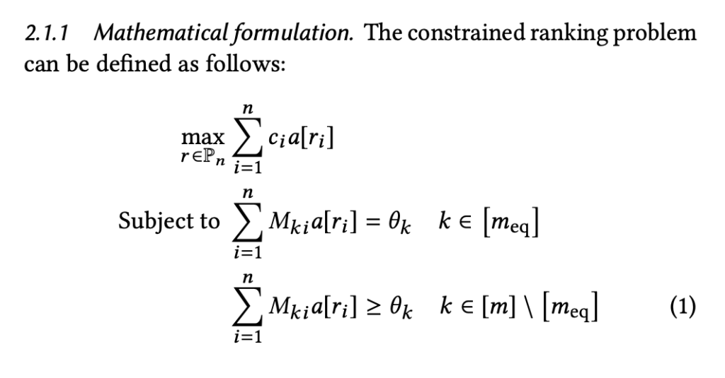
Here,  is item
  ‘s primary metric value,
  is item ‘s position after ranking
  , and
, and ![a[r_i]](https://czxttkl.com/wp-content/ql-cache/quicklatex.com-9384f0e69f08e8eb519cc02a63f47b63_l3.png "Rendered by QuickLaTeX.com") means the attention strength on each item when the item is ranked by . Similarly,
means the attention strength on each item when the item is ranked by . Similarly,  is the constraint matrix. As you can see, they define the slate reward/constraint as the sum of per-item rewards/constraints, which may or may not be the case for some application.
If there are  items, there will be
  possible rankings. Therefore, optimizing Eqn. 1 will be hard. They skillfully convert the problem into something more manageable. First, they rewrite Eqn. 1 into Eqn. 2:

 is a permutation matrix (each row and column has exactly one 1).
Then, they relax to be a probabilistic matrix,  , an “expected” permutation matrix. (In 3d, there is a typo. It should be
  ). Here,
  is a distribution for all possible permutations.
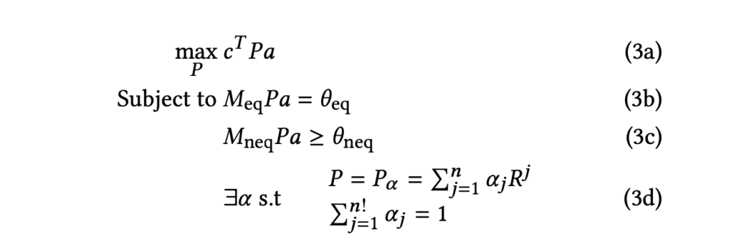
Now, we can just optimize w.r.t. , which has only  entries:

Finally, Eqn. 4 can be solved by the Lagrangian method

The rest of the paper is really complicated and hard to understand. But they are solving the same constrained optimization problem.
The second paper I read is named “Automated Creative Optimization for E-Commerce Advertising” (https://arxiv.org/abs/2103.00436). The background of this paper is that in online advertising, each candidate ads contain a set of interactive elements as a combination, such as templates, fonts, and backgrounds.

An ad’s CTR can be naturally predicted using Factorization Machine (from Eqn.3. in the paper):

The explanation for Eqn. 3 is that, there are  elements in an ads
  .
.  and
and  are the embeddings of a pair of elements, where the interaction score between the two embeddings could be computed using one of the operators, Concat, Multiply, Plus, Max, or Min. (mentioned in Section 4.2).
The problem the paper tries to solve is that when the system has many ads candidates, how can the system pick the best ads candidate believed to have the highest CTR while balancing the need to explore the element space? So they use Thompson Sampling with Bayesian Contextual Bandit. The bayesian part comes from that all embeddings (, , …) are bayesian estimates from a Gaussian distribution. For every next ads, they sample embedding values from the present distribution, pick the best ads, observe the reward, and then update the posterior distribution.

How do we update the embedding estimates  ? We use stochastic variational inference (https://czxttkl.com/2019/05/04/stochastic-variational-inference/). We can optimize with gradient-based methods w.r.t. the ELBO function, which contains only a likelihood (given a sampled
  , how likely is to observe the current dataset?) and a KL divergence between the current Gaussian distribution and a prior Gaussian distribution, both of which have an analytical expression.

This paper is a classical example of stochastic variational inference and could be applied to many real-world problems.