Evaluating trained RL policies offline is extremely important in real-world production: a trained policy with unexpected behaviors or unsuccessful learning would cause the system regress online therefore what safe to do is to evaluate their performance on the offline training data, based on which we decide whether to deploy. Evaluating policies offline is an ongoing research topic called “counterfactual policy evaluation” (CPE): what would a policy perform even though we only have trajectories that were generated by some other policy?
CPE for contextual bandit
We first look at CPE on contextual bandit problems. The contextual bandit problem is to take action  at each state
  that is drawn from a distribution
  . We can only observe the reward associated to that specific pair of and :
  . Rewards associated to other actions not taken
  can’t be observed. The next state at which you would take the next action, will not be affected by the current state or action. Essentially, contextual bandit problems are Markov Decision Problems when horizon (the number of steps) equals one. Suppose we have a dataset
  with
with  samples, each sample being a tuple
  .
.  is sampled from a behavior policy
  .
.  is calculated based on an underlying but non-observable reward function
  . For now, we ignore any noise that could exist in reward collection. To simplify our calculation, we will assume that the decision of
  is independent across samples: this assumption bypasses the possible fact that may maintain an internal memory
  , which is the history of observations used to facilitate its future decisions. We will also assume that during data collection we can access the true probability
  , the true action propensity of the behavior policy. This is not difficult to achieve in practice because we usually have the direct access to the current policy’s model. We will call the policy that we want to evaluate target policy, denoted as
  .
.
Given all these notations defined, the value function of is:
![V^{\pi_1} = \mathbb{E}_{s \sim \mathcal{D}, a \sim \pi_1(\cdot|s)}[r(s,a)]](https://czxttkl.com/wp-content/ql-cache/quicklatex.com-f4a1d1e00e97065f04cbd2ce40b97fbf_l3.png "Rendered by QuickLaTeX.com")
A straightforward way called Direct Method (DM) to estimate  is to train an approximated reward function
  and plug into :

There is one condition to be satisfied for the proof to be hold: if  then
then  . First, we don’t need to worry about that any exists in the denominator of
  because those samples would never be collected in in the first place. However, if
  for some
  , there would never be data to evaluate the outcome of taking action at state , which means becomes a biased estimator of . (Part of these ideas comes from [7].)
The intuition behind is that:
- If is a large (good) reward, and if
 , then we guess that is probably better than because may give actions leading to good rewards larger probabilities than .
- If is a small (bad) reward, and if , then we guess that is probably worse than because may give actions leading to bad rewards larger probabilities than .
- We can reverse the relationship such that if
 , we can guess is better than if itself is a bad reward. probably is a better policy trying to avoid actions leading to bad rewards.
- If and is a good reward, is probably a better policy trying to take actions leading to good rewards.
We can also relate the intuition of to Inverse Probability of Treatment Weighting (IPTW) in observational studies [5]. In observational studies, researchers want to determine the effect of certain treatment while the treatment and control selection of subjects is not totally randomized. IPTW is one kind of adjustment to observational data for measuring the treatment effect correctly. One intuitive explanation of IPTW is to weight the subject with how much information the subject could reveal [2]. For example, if a subject who has a low probability to receive treatment and has a high probability to stay in the control group happened to receive treatment, his treatment result should be very informative because he represents the characteristics mostly associated with the control group. In a similar way, we can consider the importance sampling ratio  for each as an indicator of how much information that sample reveals. When the behavior policy neglects some action that is instead emphasized by (i.e.,
  ), the sample
  has some valuable counter-factual information hence we need to “amplify” .
The third method to estimate called Doubly Robust (DR) [1] combines the direct method and IPS method:
![V^{\pi_1}_{DR}=\frac{1}{N}\sum\limits_{(s_i, a_i, r_i) \in \mathcal{S}} \big[\frac{(r_i - \hat{r}(s_i, a_i))\pi_1(a_i|s_i)}{\pi_0(a_i|s_i)} +\int\hat{r}(s_i, a')\pi_1(a'|s_i) da'\big]](https://czxttkl.com/wp-content/ql-cache/quicklatex.com-16c1ae79a43158ca6705a023d35b2d8e_l3.png "Rendered by QuickLaTeX.com")
Given our assumption that we know the true action propensity ,  is still an unbiased estimator:
![\mathbb{E}_{p_{\pi_0}(\mathcal{S})}[V^{\pi_1}_{DR}] \newline=\int p_{\pi_0}(s, a) \cdot \big[\frac{(r(s,a) - \hat{r}(s, a))\pi_1(a|s)}{\pi_0(a|s)} +\int \hat{r}(s, a')\pi_1(a'|s) da' \big]ds da \newline=\int p_{\pi_0}(s,a) \cdot\big[\frac{(r(s,a) - \hat{r}(s, a))\pi_1(a|s)}{\pi_0(a|s)} +\int(\hat{r}(s, a') - r(s,a'))\pi_1(a'|s)da' +\int r(s, a')\pi_1(a'|s)da' \big] dsda\newline=\int p_{\pi_1}(s,a) \cdot (-1+1)dsda + \int p_{\pi_1}(s,a) r(s,a) dsda\newline=V^{\pi_1}](https://czxttkl.com/wp-content/ql-cache/quicklatex.com-5b2eddcbd24d5f73844ceadc1403863d_l3.png "Rendered by QuickLaTeX.com")
However, in the original paper of DR [1], the authors don’t assume that the true action propensity can be accurately obtained. This means, can be a biased estimator: however, if  or have biases under certain bounds, would have far lower bias than either of the other two.
Under the same assumption that the true action propensity is accessible, we could get the variances of DM, DR, and IPS CPE (![Var[V^{\pi_1}_{DM}]](https://czxttkl.com/wp-content/ql-cache/quicklatex.com-12aee5da684ae437aa1a26c635fd139b_l3.png "Rendered by QuickLaTeX.com") ,
, ![Var[V^{\pi_1}_{DR}]](https://czxttkl.com/wp-content/ql-cache/quicklatex.com-8e13f1d57c52b4dffceb24ccea350b4d_l3.png "Rendered by QuickLaTeX.com") , and
, and ![Var[V^{\pi_1}_{IPS}]](https://czxttkl.com/wp-content/ql-cache/quicklatex.com-b5322ee77892dbe58ae427c62ac99361_l3.png "Rendered by QuickLaTeX.com") ) based on the formulas given in Theorem 2 in [1] while setting
) based on the formulas given in Theorem 2 in [1] while setting  because we assume we know the true action propensity:
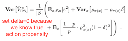
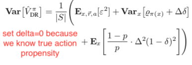
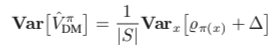
Under some reasonable assumptions according to [1], should be between and . Therefore, should be overall favored because of its zero bias and intermediate variance.
CPE for MDP
We have completed introducing several CPE methods on contextual bandit problems. Now, we move our focus to CPE on Markov Decision Problems when horizon is larger than 1. The value function of a policy is:
![V^{\pi} = \mathbb{E}_{s_0 \sim \mathcal{D}, a_t \sim \pi(\cdot|s_t), s_{t+1}\sim P(\cdot|a_t, s_t)}[\sum\limits_{t=1}^H\gamma^{t-1}r_t],](https://czxttkl.com/wp-content/ql-cache/quicklatex.com-bfc55bc4eff25229d7795708eb741006_l3.png "Rendered by QuickLaTeX.com")
where  is the number of steps in one trajectory. Simplifying the notation of this formula, we get:
![V^{\pi} = \mathbb{E}_{\tau \sim (\pi, \mu)}[R(\tau)],](https://czxttkl.com/wp-content/ql-cache/quicklatex.com-e5c9a9a941f327d049ea0a128cc6e56f_l3.png "Rendered by QuickLaTeX.com")
where  is a single trajectory,
  denotes the transition dynamics,
  is the accumulative discounted rewards for the trajectory .
Following the idea of IPS, we can have importance-sampling based CPE of based on trajectories generated by :


 is an unbiased estimator of given the same condition satisfied in : if then .
  is also an unbiased estimator of proved in [6]. However, has lower upper bound than therefore in practice usually enjoys lower variance than (compare chapter 3.5 and 3.6 in [9]).
Following the idea of DR, [3] proposed unbiased DR-based CPE on finite horizons, and later [8] extended to the infinite-horizon case:

where  and
and  are the learned q-value and value function under the behavior policy .
  and we define the corner case
  .
.
Based on Theorem 1 in [3], should have lower variance than ![Var[V^{\pi_1}_{per-decision-IS}]](https://czxttkl.com/wp-content/ql-cache/quicklatex.com-b0bf550ee2c92e20f6b532ef1f593f34_l3.png "Rendered by QuickLaTeX.com") , after realizing that per-decision-IS CPE is a special case of DR CPE.
, after realizing that per-decision-IS CPE is a special case of DR CPE.
Another CPE method also proposed by [6] is called Weighted Doubly Robust (WDR). It normalizes  in :
in :

where  .
.
 is a biased estimator but since it truncates the range of
  in to
in to ![[0,1]](https://czxttkl.com/wp-content/ql-cache/quicklatex.com-3c2f548a134dfa658b30df58bb768060_l3.png "Rendered by QuickLaTeX.com") , WDR could lower variance than DR when fewer samples are available. The low variance of WDR produces larger reduction in expected square error than the additional error incurred by the bias. (See chapter 3.8 of [9]). Furthermore, under reasonable assumptions WDR is a consistent estimator so the bias will become less an issue as the sample size increase. (As a side note, an estimator can be any combination of biased/unbiased and inconsistent/consistent [10].)
, WDR could lower variance than DR when fewer samples are available. The low variance of WDR produces larger reduction in expected square error than the additional error incurred by the bias. (See chapter 3.8 of [9]). Furthermore, under reasonable assumptions WDR is a consistent estimator so the bias will become less an issue as the sample size increase. (As a side note, an estimator can be any combination of biased/unbiased and inconsistent/consistent [10].)
Direct Method CPE on trajectories learns to reconstruct the MDP. This means DM needs to learn the transition function and reward function for simulating episodes.The biggest concern is whether the collected samples support to train a low bias model. If they do, then DM can actually achieve very good performance. [8] Section 6 lists a situation when DM can outperform DR and WDR: while DM has a low variance and low bias (even no bias), stochasticity of reward and state transition produces high variance in DR and WDR.
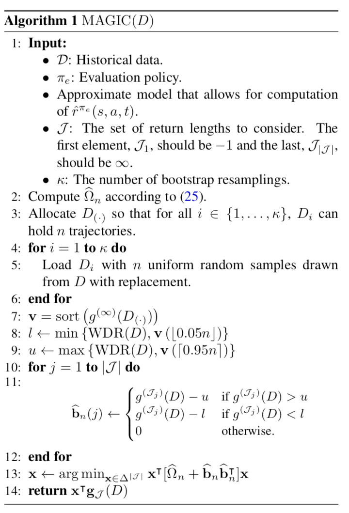
The last CPE method is called Model and Guided Importance Sampling Combining (MAGIC) [8]. It is considered as the best CPE method because it adopts the advantages from both WDR and DM. The motivation given by [8] is that CPE methods involving importance sampling are generally consistent (i.e., when samples increase, the estimated distribution moves close to the true value) but still suffer high variance; model-based methods (DM) has low variance but is biased. MAGIC combines the ideas of DM and WDR such that MAGIC can track the performance of whichever is better between DM and WDR. The MAGIC method is heavily math involved. Without deep dive into it yet, we only show its pseudocode for now:
Below is a table concluding this post, showing whether each CPE method (for evaluating trajectories) is biased/unbiased and consistent/inconsistent.
| DM |
biased |
inconsistent |
1 |
| trajectory-IS |
unbiased |
consistent |
5 |
| per-decision-IS |
unbiased |
consistent |
4 |
| DR |
unbiased |
consistent |
3 |
| WDR |
biased |
consistent |
2 |
| MAGIC |
biased |
consistent |
Not sure, possibly
between 1 and 2 |
(Table note: (1) variance rank 1 means the lowest variance, 5 means the highest; (2) when generating this table, we use some reasonable assumptions we mentioned and used in the papers cited .)
References
[1] Dudík, M., Langford, J., & Li, L. (2011, June). Doubly robust policy evaluation and learning. In Proceedings of the 28th International Conference on International Conference on Machine Learning (pp. 1097-1104). Omnipress.
[2] https://stats.stackexchange.com/questions/273367/intuitive-explanation-for-inverse-probability-of-treatment-weights-iptws-in-pr
[3] Jiang, N., & Li, L. (2016, June). Doubly robust off-policy value evaluation for reinforcement learning. In Proceedings of the 33rd International Conference on International Conference on Machine Learning-Volume 48 (pp. 652-661). JMLR. org.
[4] http://www.cs.cornell.edu/courses/cs7792/2016fa/lectures/03-counterfactualmodel_6up.pdf
[5] Austin, P. C. (2011). An introduction to propensity score methods for reducing the effects of confounding in observational studies. Multivariate behavioral research, 46(3), 399-424.
[6] Precup, D. (2000). Eligibility traces for off-policy policy evaluation. Computer Science Department Faculty Publication Series, 80.
[7] Thomas, P. S., Theocharous, G., & Ghavamzadeh, M. (2015, February). High-confidence off-policy evaluation. In Twenty-Ninth AAAI Conference on Artificial Intelligence.
[8] Thomas, P., & Brunskill, E. (2016, June). Data-efficient off-policy policy evaluation for reinforcement learning. In International Conference on Machine Learning (pp. 2139-2148).
[9] Thomas, P. S. (2015). Safe reinforcement learning (Doctoral dissertation, University of Massachusetts Libraries).
[10] https://stats.stackexchange.com/questions/31036/what-is-the-difference-between-a-consistent-estimator-and-an-unbiased-estimator
 can be multi-dimensional).
![Q_{t+1}(s_t, a_t) = (1-\alpha(s_t, a_t))Q_t(s_t, a_t) + \alpha_t(s_t, a_t)[r_t +\gamma \max_{b \in \mathcal{A}}Q_t(s_{t+1}, b)]](https://czxttkl.com/wp-content/ql-cache/quicklatex.com-d9e1d375fa70801a1e3ab636c25fdcc1_l3.png "Rendered by QuickLaTeX.com")
 from both sides and letting
  , we have:
![\triangle_t(s_t,a_t)\newline=(1-\alpha_t(s_t, a_t))\triangle_t(s_t, a_t) + \alpha_t(s,a)[r_t + \gamma\max_{b\in \mathcal{A}}Q_t(s_{t+1}, b) - Q^*(s_t, a_t)]\newline=(1-\alpha_t(s_t, a_t))\triangle_t(s_t, a_t) + \alpha_t(s_t, a_t)F_t(s_t,a_t)](https://czxttkl.com/wp-content/ql-cache/quicklatex.com-a4bd0cd1322d0e6aad3dcc206774cae9_l3.png "Rendered by QuickLaTeX.com")
 , the learning rate, to be zero for
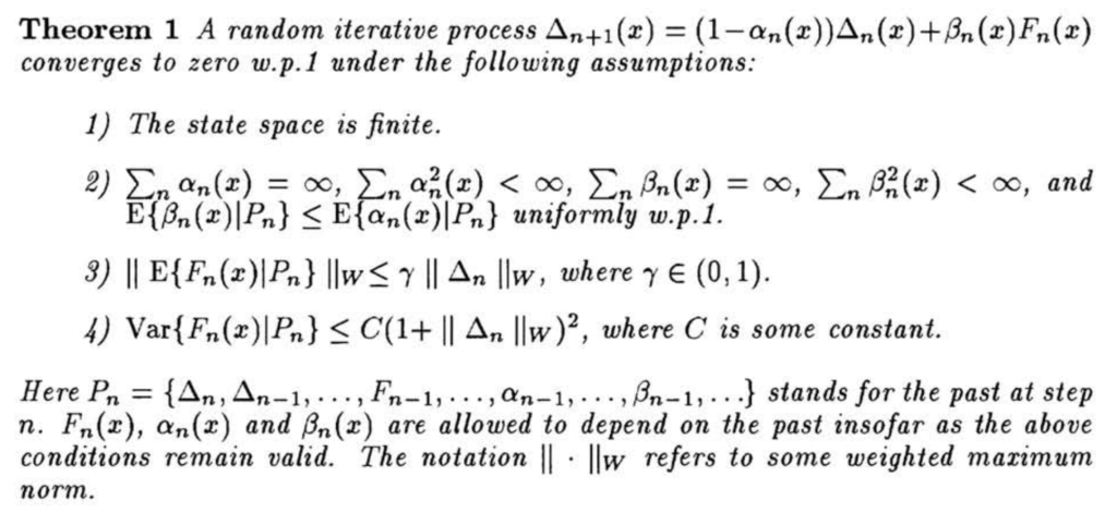
  . Till this point, we have modeled the Q-learning process exactly as the random iterative process stated in Theorem 1. Hence, as long as we can prove the 4 assumptions are held, we can prove Q-learning converges to the optimal Q-values (i.e.,
  converges to 0).
 based on our formulation. If we apply a GLIE learning policy (“greedy in the limit with infinite exploration”) [2], then we make assumption 2 hold:
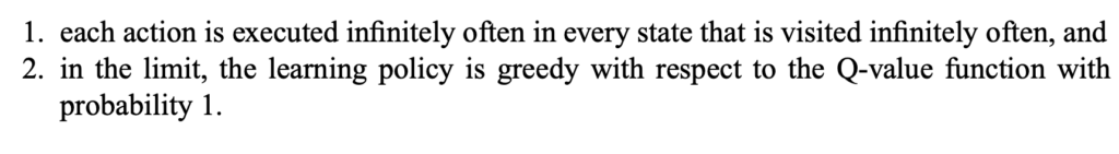
 . There are some notations that may not look familiar to ordinary audience. First,
  means the weighted maximum norm [5]. Therefore,
  . Second,
  just means
  can be estimated using all the past interactions, i.e.,
  in
in  .
. ![Q^*(s,a)=\sum\limits_{s'\in\mathcal{S}}P_a(s,s')[r(s,a,s')+\gamma \max\limits_{a'\in\mathcal{A}}Q^*(s',a')]](https://czxttkl.com/wp-content/ql-cache/quicklatex.com-d5c05af23f8d0c7487a0f957147f3c8b_l3.png "Rendered by QuickLaTeX.com")
 is a fix point of a contraction operator
  , defined over a generic function
  :
:![(\textbf{H}q)(s,a)=\sum\limits_{s'\in\mathcal{S}}P_a(s, s')[r(s,a,s')+\gamma \max\limits_{a' \in \mathcal{A}}q(s',a')]](https://czxttkl.com/wp-content/ql-cache/quicklatex.com-05808b848f849628b714664d772f3f6e_l3.png "Rendered by QuickLaTeX.com")
 , a
, a  -contraction, because:
![\|\textbf{H}q_1 - \textbf{H}q_2\|_\infty \newline=\max\limits_{s,a} \big|\sum\limits_{s'\in \mathcal{S}} P_a(s,s')[r(s,a,s')+\gamma\max\limits_{a' \in \mathcal{A}}q_1(s',a') - r(s,a, s')-\gamma \max\limits_{a'\in\mathcal{A}}q_2(s',a')]\big|\newline=\max\limits_{s,a}\gamma \big|\sum\limits_{s'\in\mathcal{S}}P_a(s,s') [\max\limits_{a' \in \mathcal{A}}q_1(s',a')-\max\limits_{a' \in \mathcal{A}}q_2(s',a')]\big|\newline\text{Think of }\max |\textbf{p}*\textbf{x}| \leq \max|p_1\cdot\max|\textbf{x}|, p_2\cdot \max|\textbf{x}|, \cdots| \text{ if } \textbf{p}>0\newline\leq\max\limits_{s,a}\gamma \sum\limits_{s'\in \mathcal{S}}P_a(s,s')\big|\max\limits_{a' \in \mathcal{A}}q_1(s',a')-\max\limits_{a' \in \mathcal{A}}q_2(s',a')\big|\newline\text{norm property: }|\textbf{u}-\textbf{v}|_\infty \geq |\textbf{u}|_\infty-|\textbf{v}|_\infty\newline\leq \max\limits_{s,a}\gamma \sum\limits_{s'\in \mathcal{S}}P_a(s,s')\max\limits_{a' \in \mathcal{A}}\big|q_1(s',a')-q_2(s',a')\big| \newline \text{Enlarge the domain of max} \newline\leq \max\limits_{s,a}\gamma \sum\limits_{s'\in \mathcal{S}}P_a(s,s')\max\limits_{s'' \in \mathcal{S},a'' \in \mathcal{A}}\big|q_1(s'',a'')-q_2(s'',a'')\big|\newline=\max\limits_{s,a}\gamma \sum\limits_{s'\in \mathcal{S}}P_a(s,s')\|q_1-q_2\|_\infty\newline=\gamma \|q_1-q_2\|_\infty](https://czxttkl.com/wp-content/ql-cache/quicklatex.com-3d90ea69364bba6dcb0961b4034592b0_l3.png "Rendered by QuickLaTeX.com")
 closer and closer to the fixed point
  at the rate of
  (in terms of L2 norm) is that the distance between
  and
and  is closer after applying
![\|E\{F_t(s,a) | P_n\}\|_w \newline=\sum\limits_{s'\in\mathcal{S}}P_a(s,s')[r(s,a,s')+\gamma\max\limits_{a'\in\mathcal{A}}Q_t(s', a')-Q^*(s,a)]\newline=\sum\limits_{s'\in\mathcal{S}}P_a(s,s')[r(s,a,s')+\gamma\max\limits_{a'\in\mathcal{A}}Q_t(s', a')]-Q^*(s,a)\newline=(\textbf{H}Q_t)(s,a)-Q^*(s,a)\newline\text{Using the fact that }Q^*=\textbf{H}Q^*\newline=(\textbf{H}Q_t)(s,a)-(\textbf{H}Q^*)(s,a)\newline \leq \|\textbf{H}Q_t-\textbf{H}Q^*\|_\infty\newline\leq \gamma \|Q_t-Q^*\|_\infty\newline=\gamma \|\triangle_t\|_\infty](https://czxttkl.com/wp-content/ql-cache/quicklatex.com-e17fe7f973a6af8acded5c30b86cc38f_l3.png "Rendered by QuickLaTeX.com")
![\[loss = -[target * log(\sigma(input)) + (1-target) * log(1 - \sigma(input))]\]](https://czxttkl.com/wp-content/ql-cache/quicklatex.com-f5c3375c9e883e92eb9e6d79f0bdcbb2_l3.png "Rendered by QuickLaTeX.com")
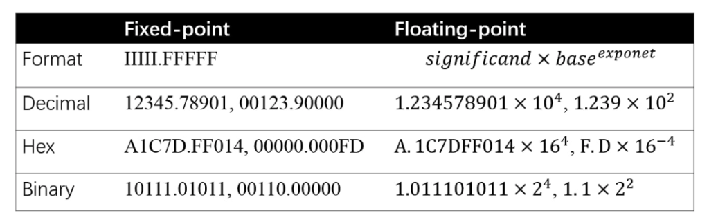
 so significand and exponent are saved as two separate numbers. Note that the precision between two consecutive floating-point numbers is not fixed but actually depends on exponents. For every exponent, the number of representable floating-point numbers is the same. But for a smaller exponent, the density of representable floating-point numbers is high; while for a larger exponent, the density is low. As a result, the closer a real value number is to 0, the more accurate it can be represented as a floating-point number. In practice, floating-point numbers are quite accurate and precise even with the largest exponent.
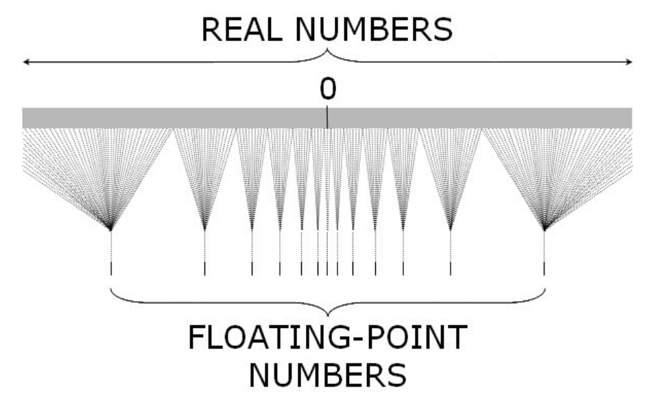
 in the equations) to make sure every FP32 can fall into INT8’s value range
 ![[0, 255]](https://czxttkl.com/wp-content/ql-cache/quicklatex.com-d19efe2d99bac51355042c3a1c252da3_l3.png "Rendered by QuickLaTeX.com") .
.
 . We have training data
  , is:
, is:![\[ H_{log p(x|\theta)} = \begin{bmatrix} \frac{\partial^2 logp(x|\theta)}{\partial \theta_1^2} & \dots & \frac{\partial^2 logp(x|\theta)}{\partial \theta_1 \partial \theta_n} \\ \dots & \dots & \dots \\ \frac{\partial^2 logp(x|\theta)}{\partial \theta_n \partial \theta_1} & \dots & \frac{\partial^2 logp(x|\theta)}{\partial \theta_n^2} \end{bmatrix} \]](https://czxttkl.com/wp-content/ql-cache/quicklatex.com-1b696b9ea8a448050586fb02d3a29092_l3.png "Rendered by QuickLaTeX.com")
 is defined as the covariance matrix of
  (note that
  , then
 ![F=\mathbb{E}_{p(x|\theta)}\left[\left(s(\theta) - mean(s(\theta))\right)\left(s(\theta) - mean(s(\theta))\right)^T\right]=\mathbb{E}_{p(x|\theta)}\left[s(\theta)s(\theta)^T\right]](https://czxttkl.com/wp-content/ql-cache/quicklatex.com-dca8e1a3d6c7f089e83a76ae6e5add5b_l3.png "Rendered by QuickLaTeX.com") . The last equation holds because
. The last equation holds because  is 0 [1]. It can be shown that the negative of
 ![\mathbb{E}_{p(x|\theta)}[H_{log p(x|\theta}]](https://czxttkl.com/wp-content/ql-cache/quicklatex.com-ab921f4d81dc1d1508717384f4234332_l3.png "Rendered by QuickLaTeX.com") is Fisher information matrix [1]. Therefore, Fisher information matrix can be thought as the (negative) curvature of log likelihood. The curvature (Hessian) of a function is the second-order derivative of the function, which depicts how quickly the gradient of the function changes. Computing Hessian (curvature) takes longer time than computing just gradient but knowing Hessian can accelerate learning convergence. If the curvature is high, the gradient changes quickly, then the gradient update of the parameters should be more cautious (i.e., smaller step); if the curvature is low, the gradient doesn’t change much, then the gradient update can be more aggressive (i.e., large step). Moreover, the eigenvalues of a Hessian determines convergence speed [3]. Therefore, knowing Fisher information matrix is quite important in optimizing a function.
is Fisher information matrix [1]. Therefore, Fisher information matrix can be thought as the (negative) curvature of log likelihood. The curvature (Hessian) of a function is the second-order derivative of the function, which depicts how quickly the gradient of the function changes. Computing Hessian (curvature) takes longer time than computing just gradient but knowing Hessian can accelerate learning convergence. If the curvature is high, the gradient changes quickly, then the gradient update of the parameters should be more cautious (i.e., smaller step); if the curvature is low, the gradient doesn’t change much, then the gradient update can be more aggressive (i.e., large step). Moreover, the eigenvalues of a Hessian determines convergence speed [3]. Therefore, knowing Fisher information matrix is quite important in optimizing a function. . The normal gradient update is:
  . The natural gradient has a little different form:
  . The natural gradient formula is actually derived from [5]:
![\[ \nabla_\theta^{NAT} \mathcal{L}(x,\theta) = \arg\min_{d} \mathcal{L}(x, \theta+d), \quad s.t. \quad KL\left( p(x|\theta) || p(x|\theta+d)\right) = c \]](https://czxttkl.com/wp-content/ql-cache/quicklatex.com-1e11c3f7669826a1e95071c279b8e9d2_l3.png "Rendered by QuickLaTeX.com")
 . Another way to think about natural gradient is that since the Fisher information matrix
  and the observation is denoted as
 is the probability of observation marginal over all possible model parameters:
 , which is what we want to know. Therefore, we need to come up with a way to approximate
  .
.  and
and  . Those representing the difference between the two distributions as Kullback-Leibler divergence is called variational inference. If we further categorize based on the family of
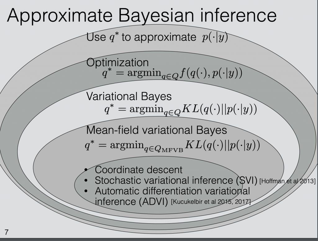
 is defined as [4]:
![KL\left(h(x)||g(x)\right)\newline=\int^\infty_{-\infty}h(x)log\frac{h(x)}{g(x)}dx \newline=\mathbb{E}_h[log\;h(x)]-\mathbb{E}_h[log\;g(x)]](https://czxttkl.com/wp-content/ql-cache/quicklatex.com-8501d9a8fd963ea67a6922b3315189d5_l3.png "Rendered by QuickLaTeX.com")
 using variational Bayes, we define the following objective function:
 ,
, ![KL(q(z)||p(z|x))=\mathbb{E}_q [log\;q(z)] - \mathbb{E}_q [log\;p(z,x)]+log\;p(x)](https://czxttkl.com/wp-content/ql-cache/quicklatex.com-20412537c9a69fb1219645c609aca19a_l3.png "Rendered by QuickLaTeX.com") . (all expectations are taken with respect to
. (all expectations are taken with respect to  , then
  can be treated as a constant. Thus, minimizing the KL-divergence is equivalent to maximizing:
![ELBO(q)=\mathbb{E}_q[log\;p(z,x)] - \mathbb{E}_q[log\;q(z)]](https://czxttkl.com/wp-content/ql-cache/quicklatex.com-44dac15424746676e23c8c9dd88b3734_l3.png "Rendered by QuickLaTeX.com")
 is the lower bound of

 and a random variable
  ,
, ![f(\mathbb{E}[X]) \leq \mathbb{E}\left[f(X)\right]](https://czxttkl.com/wp-content/ql-cache/quicklatex.com-600448c8beb2e15285d94f6085146d09_l3.png "Rendered by QuickLaTeX.com") ; for a concave function
; for a concave function  ,
, ![g(\mathbb{E}[X]) \geq \mathbb{E}\left[g(X)\right]](https://czxttkl.com/wp-content/ql-cache/quicklatex.com-b66abed9814432bc198369d55e5a7f25_l3.png "Rendered by QuickLaTeX.com") . Therefore, we have:
. Therefore, we have:![log \; p(x)\newline=log \int_z p(z,x)\newline=log \int_z p(z,x)\frac{q(z)}{q(z)}\newline=log \int_z q(z)\frac{p(z,x)}{q(z)}\newline=log \left(\mathbb{E}_{q(z)}\left[\frac{p(z,x)}{q(z)}\right]\right) \newline \geq \mathbb{E}_{q(z)}\left[log \frac{p(z,x)}{q(z)}\right] \quad\quad \text{by Jensen's inequality} \newline =ELBO(q)](https://czxttkl.com/wp-content/ql-cache/quicklatex.com-24349341ab84453e6b667fde54e71db3_l3.png "Rendered by QuickLaTeX.com")

![ELBO(q)\newline=\mathbb{E}_q[log\;p(z,x)] - \mathbb{E}_q[log\;q(z)]\newline=\mathbb{E}_q[log\;p(x|z)] + \mathbb{E}_q[log\;p(z)] - \mathbb{E}_q[log\;q(z)] \quad\quad p(z) \text{ is the prior of } z \newline= \mathbb{E}_q[log\;p(x|z)] - \mathbb{E}_q [log \frac{q(z)}{p(z)}]\newline=\mathbb{E}_q[log\;p(x|z)] - KL\left(q(z) || p(z)\right)](https://czxttkl.com/wp-content/ql-cache/quicklatex.com-aa0eccc6fce4b2b3085999bb67659a1f_l3.png "Rendered by QuickLaTeX.com")
 . The second part encourages
  .
.  . In practice, minimizing with regard to
 . Hence, the objective function to approximate
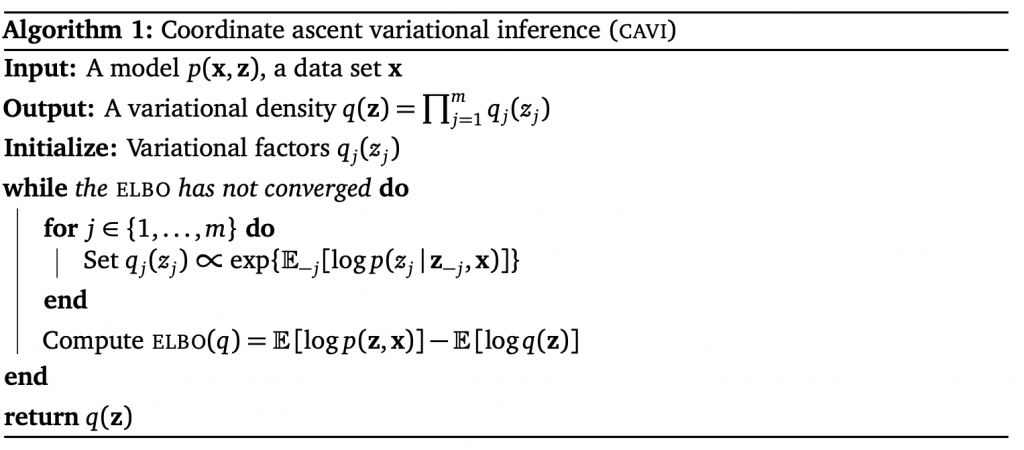
![q_j(z_j) \propto exp\{\mathbb{E}_{-j}[log p(z_j|z_{-j}, x)]\}](https://czxttkl.com/wp-content/ql-cache/quicklatex.com-8363d2aec9de7b037c19991a7105feb8_l3.png "Rendered by QuickLaTeX.com") ” may seems hard to understand. It means that setting the variational distribution parameter
” may seems hard to understand. It means that setting the variational distribution parameter  follows the distribution that is equivalent to
 ![exp\{\mathbb{E}_{-j}[log p(z_j|z_{-j}, x)]\}](https://czxttkl.com/wp-content/ql-cache/quicklatex.com-df13519a244296cb5ca9b9f499b32134_l3.png "Rendered by QuickLaTeX.com") up to a constant.
up to a constant.  means that the expectation is taken with regard to a distribution
  .
. ?
? or sample
  . One thing to note is that there is no restriction on the parametric form of the individual variational distribution. For example, you may define
  . Then, the mean of
  . If
. If  and use it to update
  , where
  ,
,  , and
, and  are defined according to the definition of the exponential family [10].
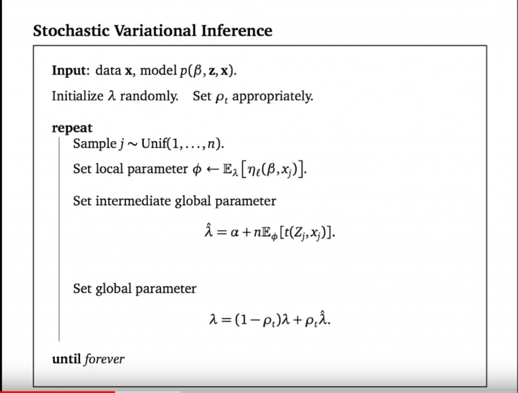
 that fit the formula:
  . If we assume normality of the errors:
  with a fixed point estimate on
  , we could also enable analysis on confidence interval and future prediction (see discussion in the end of [2]). Instead of point estimates, bayesian linear regression assumes
 represents observed data
  and
and 

 and variance
  .
. , we usually require that the prior in the same probability distribution family as the likelihood. Here we can treat the likelihood
  as a two-dimensional exponential family (the concept is illustrated in chapter 4 in [6]), a distribution regarding to
  , can be modeled as a Normal-inverse-Gamma (NIG) distribution:
 is also called inverse chi-squared distribution; they only differ in parameterization [9]. We can denote
  . Note that we express
  , meaning that
  , we would not get a conjugate prior. Second, if you think
  are generated from some process governed by
  ,
,


![\mathbb{E}_{p_{\pi_0}(\mathcal{S})}[V^{\pi_1}_{IPS}] \newline (p_{\pi_0}(\mathcal{S}) \text{ is the joint distribution of all samples generated by }\pi_0) \newline = \frac{1}{N}\int p_{\pi_0}(\mathcal{S})\sum\limits_{(s_i, a_i, r_i) \in \mathcal{S}} \frac{r_i \pi_1(a_i|s_i)}{\pi_0(a_i|s_i)} d\mathcal{S} \newline \text{(since each sample is collected independently, we have:)}\newline=\frac{1}{N}\sum\limits_{(s_i, a_i, r_i) \in \mathcal{S}}\int p_{\pi_0}(s_i, a_i)\frac{r(s_i, a_i)\pi_1(a_i|s_i)}{\pi_0(a_i|s_i)}ds_i da_i \newline=\int p_{\pi_0}(s, a)\frac{r(s, a)\pi_1(a|s)}{\pi_0(a|s)}ds da \newline=\int p_\mathcal{D}(s) \pi_0(a|s)\frac{r(s, a)\pi_1(a|s)}{\pi_0(a|s)}dsda \newline=\int p_{\pi_1}(s,a)r(s,a) dsda\newline=V^{\pi_1}](https://czxttkl.com/wp-content/ql-cache/quicklatex.com-bb82f8b47ba652b49135c45939d0b150_l3.png "Rendered by QuickLaTeX.com")