Counterfactual Policy Evaluation

Evaluating trained RL policies offline is extremely important in real-world production: a trained policy with unexpected behaviors or unsuccessful learning would cause the system regress online therefore what safe to do is to evaluate their performance on the offline training data, based on which we decide whether to deploy. Evaluating policies offline is an ongoing research topic called “counterfactual policy evaluation” (CPE): what would a policy perform even though we only have trajectories that were generated by some other policy?

CPE for contextual bandit

We first look at CPE on contextual bandit problems. The contextual bandit problem is to take action $a$ at each state $s$ that is drawn from a distribution $\mathcal{D}$ . We can only observe the reward associated to that specific pair of $s$ and $a$ : $r(s, a)$ . Rewards associated to other actions not taken $r(s,a'), a' \neq a$ can’t be observed. The next state at which you would take the next action, will not be affected by the current state or action. Essentially, contextual bandit problems are Markov Decision Problems when horizon (the number of steps) equals one. Suppose we have a dataset $\mathcal{S}$ with $N$ samples, each sample being a tuple $(s_i, a_i, r_i), i=1,2,\cdots,N$ . $a_i$ is sampled from a behavior policy $\pi_0(a|s)$ . $r_i$ is calculated based on an underlying but non-observable reward function $r_i=r(s_i, a_i)$ . For now, we ignore any noise that could exist in reward collection. To simplify our calculation, we will assume that the decision of $\pi_0$ is independent across samples: this assumption bypasses the possible fact that $\pi_0$ may maintain an internal memory $h$ , which is the history of observations used to facilitate its future decisions. We will also assume that during data collection we can access the true probability $\pi_0(\cdot|s)$ , the true action propensity of the behavior policy. This is not difficult to achieve in practice because we usually have the direct access to the current policy’s model. We will call the policy that we want to evaluate target policy, denoted as $\pi_1$ .

Given all these notations defined, the value function of $\pi_1$ is:

$V^{\pi_1} = \mathbb{E}_{s \sim \mathcal{D}, a \sim \pi_1(\cdot|s)}[r(s,a)]$

A straightforward way called Direct Method (DM) to estimate $V^{\pi_1}$ is to train an approximated reward function $\hat{r}$ and plug into $V^{\pi_1}$ :

$V^{\pi_1}_{DM}=\frac{1}{N}\sum\limits_{s \in \mathcal{S}}\sum\limits_a \hat{r}(s,a)\pi_1(a|s)$

The bias of $\hat{r}$ directly determines the bias of $V^{\pi_1}_{DM}$ . The problem is that if $\hat{r}$ is only trained on $\mathcal{S}$ generated by $\pi_0$ , it might be possible that these samples do not sufficiently cover state/action pairs relevant to $V^{\pi_1}$ , thus $\hat{r}$ could be very biased and inaccurate.

The second method is called inverse propensity score (IPS). Its formulation is basically importance sampling on rewards:

$V^{\pi_1}_{IPS} = \frac{1}{N} \sum\limits_{(s_i, a_i, r_i) \in \mathcal{S}} \frac{r_i \pi_1(a_i|s_i)}{\pi_0(a_i|s_i)}$

We can prove that $V^{\pi_1}_{IPS}$ is an unbiased estimator of $V^{\pi_1}$ . I get some ideas from [4]:

$\mathbb{E}_{p_{\pi_0}(\mathcal{S})}[V^{\pi_1}_{IPS}] \newline (p_{\pi_0}(\mathcal{S}) \text{ is the joint distribution of all samples generated by }\pi_0) \newline = \frac{1}{N}\int p_{\pi_0}(\mathcal{S})\sum\limits_{(s_i, a_i, r_i) \in \mathcal{S}} \frac{r_i \pi_1(a_i|s_i)}{\pi_0(a_i|s_i)} d\mathcal{S} \newline \text{(since each sample is collected independently, we have:)}\newline=\frac{1}{N}\sum\limits_{(s_i, a_i, r_i) \in \mathcal{S}}\int p_{\pi_0}(s_i, a_i)\frac{r(s_i, a_i)\pi_1(a_i|s_i)}{\pi_0(a_i|s_i)}ds_i da_i \newline=\int p_{\pi_0}(s, a)\frac{r(s, a)\pi_1(a|s)}{\pi_0(a|s)}ds da \newline=\int p_\mathcal{D}(s) \pi_0(a|s)\frac{r(s, a)\pi_1(a|s)}{\pi_0(a|s)}dsda \newline=\int p_{\pi_1}(s,a)r(s,a) dsda\newline=V^{\pi_1}$

There is one condition to be satisfied for the proof to be hold: if $\pi_0(a|s)=0$ then $\pi_1(a|s)=0$ . First, we don’t need to worry about that any $\pi_0(a|s)=0$ exists in the denominator of $V^{\pi_1}_{IPS}$ because those samples would never be collected in $\mathcal{S}$ in the first place. However, if $\pi_0(a|s)=0, \pi_1(a|s)>0$ for some $(s,a)$ , there would never be data to evaluate the outcome of taking action $a$ at state $s$ , which means $V^{\pi_1}_{IPS}$ becomes a biased estimator of $V^{\pi_1}$ . (Part of these ideas comes from [7].)

The intuition behind $V^{\pi_1}_{IPS}$ is that:

If $r_i$ is a large (good) reward, and if $\pi_1(a_i|s_i) > \pi_0(a_i|s_i)$ , then we guess that $\pi_1$ is probably better than $\pi_0$ because $\pi_1$ may give actions leading to good rewards larger probabilities than $\pi_0$ .
If $r_i$ is a small (bad) reward, and if $\pi_1(a_i|s_i) > \pi_0(a_i|s_i)$ , then we guess that $\pi_1$ is probably worse than $\pi_0$ because $\pi_1$ may give actions leading to bad rewards larger probabilities than $\pi_0$ .
We can reverse the relationship such that if $\pi_1(a_i|s_i) < \pi_0(a_i|s_i)$ , we can guess $\pi_1$ is better than $\pi_0$ if $r_i$ itself is a bad reward. $\pi_1$ probably is a better policy trying to avoid actions leading to bad rewards.
If $\pi_1(a_i|s_i) < \pi_0(a_i|s_i)$ and $r_i$ is a good reward, $\pi_0$ is probably a better policy trying to take actions leading to good rewards.

We can also relate the intuition of $V^{\pi_1}_{IPS}$ to Inverse Probability of Treatment Weighting (IPTW) in observational studies [5]. In observational studies, researchers want to determine the effect of certain treatment while the treatment and control selection of subjects is not totally randomized. IPTW is one kind of adjustment to observational data for measuring the treatment effect correctly. One intuitive explanation of IPTW is to weight the subject with how much information the subject could reveal [2]. For example, if a subject who has a low probability to receive treatment and has a high probability to stay in the control group happened to receive treatment, his treatment result should be very informative because he represents the characteristics mostly associated with the control group. In a similar way, we can consider the importance sampling ratio $\frac{\pi_1(a_i|s_i)}{\pi_0(a_i|s_i)}$ for each $r_i$ as an indicator of how much information that sample reveals. When the behavior policy $\pi_0$ neglects some action $a_i$ that is instead emphasized by $\pi_1$ (i.e., $\pi_0(a_i|s_i) < \pi_1(a_i|s_i)$ ), the sample $(s_i, a_i, r_i)$ has some valuable counter-factual information hence we need to “amplify” $r_i$ .

The third method to estimate $V^{\pi_1}$ called Doubly Robust (DR) [1] combines the direct method and IPS method:

$V^{\pi_1}_{DR}=\frac{1}{N}\sum\limits_{(s_i, a_i, r_i) \in \mathcal{S}} \big[\frac{(r_i - \hat{r}(s_i, a_i))\pi_1(a_i|s_i)}{\pi_0(a_i|s_i)} +\int\hat{r}(s_i, a')\pi_1(a'|s_i) da'\big]$

Given our assumption that we know the true action propensity $\pi_0(\cdot|s)$ , $V^{\pi_1}_{DR}$ is still an unbiased estimator:

$\mathbb{E}_{p_{\pi_0}(\mathcal{S})}[V^{\pi_1}_{DR}] \newline=\int p_{\pi_0}(s, a) \cdot \big[\frac{(r(s,a) - \hat{r}(s, a))\pi_1(a|s)}{\pi_0(a|s)} +\int \hat{r}(s, a')\pi_1(a'|s) da' \big]ds da \newline=\int p_{\pi_0}(s,a) \cdot\big[\frac{(r(s,a) - \hat{r}(s, a))\pi_1(a|s)}{\pi_0(a|s)} +\int(\hat{r}(s, a') - r(s,a'))\pi_1(a'|s)da' +\int r(s, a')\pi_1(a'|s)da' \big] dsda\newline=\int p_{\pi_1}(s,a) \cdot (-1+1)dsda + \int p_{\pi_1}(s,a) r(s,a) dsda\newline=V^{\pi_1}$

However, in the original paper of DR [1], the authors don’t assume that the true action propensity can be accurately obtained. This means, $V^{\pi_1}_{DR}$ can be a biased estimator: however, if $V^{\pi_1}_{DM}$ or $V^{\pi_1}_{IPS}$ have biases under certain bounds, $V^{\pi_1}_{DR}$ would have far lower bias than either of the other two.

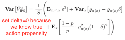
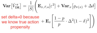
Under the same assumption that the true action propensity is accessible, we could get the variances of DM, DR, and IPS CPE ( $Var[V^{\pi_1}_{DM}]$ , $Var[V^{\pi_1}_{DR}]$ , and $Var[V^{\pi_1}_{IPS}]$ ) based on the formulas given in Theorem 2 in [1] while setting $\delta=0$ because we assume we know the true action propensity:

ips

Under some reasonable assumptions according to [1], $Var[V^{\pi_1}_{DR}]$ should be between $Var[V^{\pi_1}_{DM}]$ and $Var[V^{\pi_1}_{IPS}]$ . Therefore, $V^{\pi_1}_{DR}$ should be overall favored because of its zero bias and intermediate variance.

CPE for MDP

We have completed introducing several CPE methods on contextual bandit problems. Now, we move our focus to CPE on Markov Decision Problems when horizon is larger than 1. The value function of a policy is:

$V^{\pi} = \mathbb{E}_{s_0 \sim \mathcal{D}, a_t \sim \pi(\cdot|s_t), s_{t+1}\sim P(\cdot|a_t, s_t)}[\sum\limits_{t=1}^H\gamma^{t-1}r_t],$

where $H$ is the number of steps in one trajectory. Simplifying the notation of this formula, we get:

$V^{\pi} = \mathbb{E}_{\tau \sim (\pi, \mu)}[R(\tau)],$

where $\tau$ is a single trajectory, $\mu$ denotes the transition dynamics, $R(\tau)=\sum\limits_{t=1}^H\gamma^{t-1}r_t$ is the accumulative discounted rewards for the trajectory $\tau$ .

Following the idea of IPS, we can have importance-sampling based CPE of $\pi_1$ based on trajectories generated by $\pi_0$ :

$V^{\pi_1}_{trajectory-IS}(\tau) = R(\tau) \prod\limits_{t=1}^H\frac{\pi_1(a_t|s_t)}{\pi_0(a_t|s_t)}$

$V^{\pi_1}_{per-decision-IS}(\tau)\newline=\sum\limits_{t=1}^H \gamma^{t-1} r_t \prod\limits_{j=1}^t \frac{\pi_1(a_j|s_j)}{\pi_0(a_j|s_j)}\newline=\sum\limits_{t=1}^H \gamma^{t-1} r_t \rho_{1:t}$

$V^{\pi_1}_{trajectory-IS}$ is an unbiased estimator of $V^{\pi_1}$ given the same condition satisfied in $V^{\pi_1}_{IPS}$ : if $\pi_0(a|s)=0$ then $\pi_1(a|s)=0$ . $V^{\pi_1}_{per-decision-IS}$ is also an unbiased estimator of $V^{\pi_1}$ proved in [6]. However, $V^{\pi_1}_{per-decision-IS}$ has lower upper bound than $V^{\pi_1}_{trajectory-IS}$ therefore in practice $V^{\pi_1}_{per-decision-IS}$ usually enjoys lower variance than $V^{\pi_1}_{trajectory-IS}$ (compare chapter 3.5 and 3.6 in [9]).

Following the idea of DR, [3] proposed unbiased DR-based CPE on finite horizons, and later [8] extended to the infinite-horizon case:

$V^{\pi_1}_{DR}(\tau)=\sum\limits_{t=1}^\infty \gamma^{t-1}r_t\rho_{1:t} -\sum\limits_{t=1}^\infty \gamma^{t-1} \big( \rho_{1:t}\hat{q}^{\pi_1}(s_t, a_t)-\rho_{1:t-1}\hat{v}^{\pi_1}(s_t) \big),$

where $\hat{q}^{\pi_0}$ and $\hat{v}^{\pi_0}$ are the learned q-value and value function under the behavior policy $\pi_0$ . $\rho_{1:t} = \prod\limits_{i=1}^t\frac{\pi_1(a_i|s_i)}{\pi_0(a_i|s_i)}$ and we define the corner case $\rho_{1:0} = 1$ .

Based on Theorem 1 in [3], $Var[V^{\pi_1}_{DR}]$ should have lower variance than $Var[V^{\pi_1}_{per-decision-IS}]$ , after realizing that per-decision-IS CPE is a special case of DR CPE.

Another CPE method also proposed by [6] is called Weighted Doubly Robust (WDR). It normalizes $\rho_{1:t}$ in $V^{\pi_1}_{DR}$ :

$V^{\pi_1}_{WDR}(\tau)=\sum\limits_{t=1}^\infty \gamma^{t-1}r_t w_{1:t} -\sum\limits_{t=1}^\infty \gamma^{t-1} \big( w_{1:t}\hat{q}^{\pi_1}(s_t, a_t)-w_{1:t-1}\hat{v}^{\pi_1}(s_t) \big),$

where $w_{1:t} = \frac{\rho_{1:t}}{\sum\limits_\tau \rho_{1:t}}$ .

$V^{\pi_1}_{WDR}$ is a biased estimator but since it truncates the range of $\rho$ in $V^{\pi_1}_{DR}$ to $[0,1]$ , WDR could lower variance than DR when fewer samples are available. The low variance of WDR produces larger reduction in expected square error than the additional error incurred by the bias. (See chapter 3.8 of [9]). Furthermore, under reasonable assumptions WDR is a consistent estimator so the bias will become less an issue as the sample size increase. (As a side note, an estimator can be any combination of biased/unbiased and inconsistent/consistent [10].)

Direct Method CPE on trajectories learns to reconstruct the MDP. This means DM needs to learn the transition function and reward function for simulating episodes.The biggest concern is whether the collected samples support to train a low bias model. If they do, then DM can actually achieve very good performance. [8] Section 6 lists a situation when DM can outperform DR and WDR: while DM has a low variance and low bias (even no bias), stochasticity of reward and state transition produces high variance in DR and WDR.

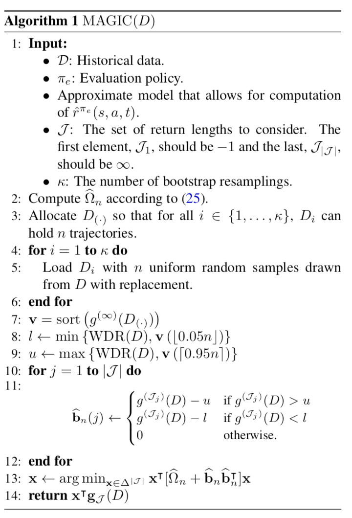
The last CPE method is called Model and Guided Importance Sampling Combining (MAGIC) [8]. It is considered as the best CPE method because it adopts the advantages from both WDR and DM. The motivation given by [8] is that CPE methods involving importance sampling are generally consistent (i.e., when samples increase, the estimated distribution moves close to the true value) but still suffer high variance; model-based methods (DM) has low variance but is biased. MAGIC combines the ideas of DM and WDR such that MAGIC can track the performance of whichever is better between DM and WDR. The MAGIC method is heavily math involved. Without deep dive into it yet, we only show its pseudocode for now:

Screen Shot 2019-02-19 at 11.26.03 PM

Below is a table concluding this post, showing whether each CPE method (for evaluating trajectories) is biased/unbiased and consistent/inconsistent.

DM	biased	inconsistent	1
trajectory-IS	unbiased	consistent	5
per-decision-IS	unbiased	consistent	4
DR	unbiased	consistent	3
WDR	biased	consistent	2
MAGIC	biased	consistent	Not sure, possibly between 1 and 2

(Table note: (1) variance rank 1 means the lowest variance, 5 means the highest; (2) when generating this table, we use some reasonable assumptions we mentioned and used in the papers cited .)

References

[1] Dudík, M., Langford, J., & Li, L. (2011, June). Doubly robust policy evaluation and learning. In Proceedings of the 28th International Conference on International Conference on Machine Learning (pp. 1097-1104). Omnipress.

[2] https://stats.stackexchange.com/questions/273367/intuitive-explanation-for-inverse-probability-of-treatment-weights-iptws-in-pr

[3] Jiang, N., & Li, L. (2016, June). Doubly robust off-policy value evaluation for reinforcement learning. In Proceedings of the 33rd International Conference on International Conference on Machine Learning-Volume 48 (pp. 652-661). JMLR. org.

[4] http://www.cs.cornell.edu/courses/cs7792/2016fa/lectures/03-counterfactualmodel_6up.pdf

[5] Austin, P. C. (2011). An introduction to propensity score methods for reducing the effects of confounding in observational studies. Multivariate behavioral research, 46(3), 399-424.

[6] Precup, D. (2000). Eligibility traces for off-policy policy evaluation. Computer Science Department Faculty Publication Series, 80.

[7] Thomas, P. S., Theocharous, G., & Ghavamzadeh, M. (2015, February). High-confidence off-policy evaluation. In Twenty-Ninth AAAI Conference on Artificial Intelligence.

[8] Thomas, P., & Brunskill, E. (2016, June). Data-efficient off-policy policy evaluation for reinforcement learning. In International Conference on Machine Learning (pp. 2139-2148).

[9] Thomas, P. S. (2015). Safe reinforcement learning (Doctoral dissertation, University of Massachusetts Libraries).

[10] https://stats.stackexchange.com/questions/31036/what-is-the-difference-between-a-consistent-estimator-and-an-unbiased-estimator