czxttkl – Page 7

Personalized Re-ranking

In the industry there is a trend to add a re-ranker at the final stage of a recommendation system. The re-ranker ranks the items that have already been filtered out from an enormous candidate set, aiming to provide the finest level of personalized ordering before the items are ultimately delivered to the user.

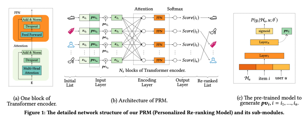
In this post I am trying to have a quick re-implementation of “Personalized Re-ranking for Recommendation” [1]. The model architecture is as follows. A transformer encoder encodes candidate item features and user features, and then attention score is computed for each item (analogous to pairwise ranking). All attention scores will pass through a softmax function and fit with click labels.

import dataclasses
from dataclasses import asdict, dataclass
import torch.nn as nn
from functools import partial, reduce
import torch
import numpy as np
from torch.utils.data import DataLoader, Dataset
import random
from typing import cast

PADDING_SYMBOL = 0

@dataclass
class PreprocessedRankingInput:
    state_features: torch.Tensor
    src_seq: torch.Tensor
    tgt_out_seq: torch.Tensor
    slate_reward: torch.Tensor
    position_reward: torch.Tensor
    tgt_out_idx: torch.Tensor
        
    def _replace(self, **kwargs):
        return cast(type(self), dataclasses.replace(self, **kwargs))

    def cuda(self):
        cuda_tensor = {}
        for field in dataclasses.fields(self):
            f = getattr(self, field.name)
            if isinstance(f, torch.Tensor):
                cuda_tensor[field.name] = f.cuda(non_blocking=True)
        return self._replace(**cuda_tensor)


def embedding_np(idx, table):
    """ numpy version of embedding look up """
    new_shape = (*idx.shape, -1)
    return table[idx.flatten()].reshape(new_shape)


class TransposeLayer(nn.Module):
    def forward(self, input):
        return input.transpose(1, 0)


def create_encoder(
    input_dim,
    d_model=512,
    nhead=2,
    dim_feedforward=512,
    dropout=0.1,
    activation="relu",
    num_encoder_layers=2,
    use_gpu=False,
):
    feat_embed = nn.Linear(input_dim, d_model)
    encoder_layer = nn.TransformerEncoderLayer(
        d_model, nhead, dim_feedforward, dropout, activation
    )
    encoder_norm = nn.LayerNorm(d_model)
    encoder = nn.TransformerEncoder(encoder_layer, num_encoder_layers, encoder_norm)
    scorer = nn.Linear(d_model, 1)
    final_encoder = nn.Sequential(
        feat_embed, 
        nn.ReLU(), 
        TransposeLayer(), # make sure batch_size is the first dim
        encoder, # nn.TransformerEncoder assumes batch_size is the second dim
        TransposeLayer(), 
        nn.ReLU(), 
        scorer
    )
    if use_gpu:
        final_encoder.cuda()
    return final_encoder


def _num_of_params(model):
    return len(torch.cat([p.flatten() for p in model.parameters()]))

def _print_gpu_mem(use_gpu):
    if use_gpu:
        print(
            'gpu usage',
            torch.cuda.memory_stats(
                torch.device('cuda')
            )['active_bytes.all.current'] / 1024 / 1024 / 1024,
            'GB',
        )

def create_nn(
    input_dim,
    d_model=512,
    nhead=8,
    dim_feedforward=512,
    dropout=0.1,
    activation="relu",
    num_encoder_layers=2,
    use_gpu=False,
):

    feat_embed = nn.Linear(input_dim, d_model)
    scorer = nn.Linear(d_model, 1)
    final_nn = nn.Sequential(
        feat_embed,
        nn.ReLU(),
        nn.Linear(d_model, d_model),
        nn.ReLU(),
        nn.Linear(d_model, d_model),
        nn.ReLU(),
        scorer,
    )
    if use_gpu:
        final_nn.cuda()
    return final_nn


def batch_to_score(encoder, batch, test=False):
    batch_size, tgt_seq_len = batch.tgt_out_idx.shape
    state_feat_dim = batch.state_features.shape[1]

    concat_feat_vec = torch.cat(
        (
            batch.state_features.repeat(1, max_src_seq_len).reshape(
                batch_size, max_src_seq_len, state_feat_dim
            ),
            batch.src_seq,
        ),
        dim=2,
    )
    encoder_output = encoder(concat_feat_vec).squeeze(-1)
    if test:
        return encoder_output

    device = encoder_output.device
    slate_encoder_output = encoder_output[
        torch.arange(batch_size, device=device).repeat_interleave(tgt_seq_len),
        batch.tgt_out_idx.flatten(),
    ].reshape(batch_size, tgt_seq_len)
    
    return slate_encoder_output


def train(encoder, batch, optimizer):
    # shape: batch_size, tgt_seq_len
    slate_encoder_output = batch_to_score(encoder, batch)

    log_softmax = nn.LogSoftmax(dim=1)
    kl_loss = nn.KLDivLoss(reduction="batchmean")
    loss = kl_loss(log_softmax(slate_encoder_output), batch.position_reward)

    optimizer.zero_grad()
    loss.backward()
    optimizer.step()

    return loss.detach().cpu().numpy()


@torch.no_grad()
def test(encoder, batch):
    encoder.eval()
    # shape: batch_size, tgt_seq_len
    slate_encoder_output = batch_to_score(encoder, batch, test=False)
    slate_acc = torch.mean(
        (
            torch.argmax(slate_encoder_output, dim=1)
            == torch.argmax(batch.position_reward, dim=1)
        ).float()
    )

    # shape: batch_size, seq_seq_len
    total_encoder_output = batch_to_score(encoder, batch, test=True)
    batch_size = batch.tgt_out_idx.shape[0]
    correct_idx = batch.tgt_out_idx[
        torch.arange(batch_size), torch.argmax(batch.position_reward, dim=1)
    ]
    total_acc = torch.mean(
        (
            torch.argmax(total_encoder_output, dim=1)
            == correct_idx
        ).float()
    )

    encoder.train()
    print(f"slate acc {slate_acc}, total acc {total_acc}")


       
class ValueModel(nn.Module):
    """
    Generate ground-truth VM coefficients based on user features + candidate distribution
    """

    def __init__(self, state_feat_dim, candidate_feat_dim, hidden_size):
        super(ValueModel, self).__init__()
        self.state_feat_dim = state_feat_dim
        self.candidate_feat_dim = candidate_feat_dim
        self.hidden_size = hidden_size
        self.layer1 = nn.Linear(state_feat_dim + 3 * candidate_feat_dim, candidate_feat_dim)
        for p in self.parameters():
            if p.dim() > 1:
                nn.init.xavier_uniform_(p)
            # model will be called with fixed parameters
            p.requires_grad = False

    def forward(
        self,
        state_features,
        src_seq,
        tgt_out_seq,
        tgt_out_idx,
    ):
        batch_size, max_src_seq_len, candidate_feat_dim = src_seq.shape
        max_tgt_seq_len = tgt_out_seq.shape[1]

        mean = src_seq.mean(dim=1)
        std = src_seq.std(dim=1)
        max = src_seq.max(dim=1).values
        vm_coef = self.layer1(torch.cat((state_features, mean, std, max), dim=1)).unsqueeze(2)
        pointwise_score = torch.bmm(tgt_out_seq, vm_coef).squeeze()
        return pointwise_score
                

class TestDataset(Dataset):
    def __init__(
        self,
        batch_size: int,
        num_batches: int,
        state_feat_dim: int,
        candidate_feat_dim: int,
        max_src_seq_len: int,
        max_tgt_seq_len: int,
        use_gpu: bool,
    ):
        self.batch_size = batch_size
        self.num_batches = num_batches
        self.state_feat_dim = state_feat_dim
        self.candidate_feat_dim = candidate_feat_dim
        self.max_src_seq_len = max_src_seq_len
        self.max_tgt_seq_len = max_tgt_seq_len
        self.use_gpu = use_gpu

        self.personalized_vm = ValueModel(state_feat_dim, candidate_feat_dim, 10)
        if use_gpu:
            self.personalized_vm.cuda()

    def __len__(self):
        return self.num_batches

    def action_generator(self, state_features, src_seq):
        batch_size, max_src_seq_len, _ = src_seq.shape
        action = np.full((batch_size, self.max_tgt_seq_len), PADDING_SYMBOL).astype(np.long)
        for i in range(batch_size):
            action[i] = np.random.permutation(
                np.arange(self.max_src_seq_len)
            )[:self.max_tgt_seq_len]
        return action

    def reward_oracle(
        self,
        state_features,
        src_seq,
        tgt_out_seq,
        tgt_out_idx,
    ):
        batch_size = state_features.shape[0]
        # shape: batch_size x max_tgt_seq_len
        pointwise_score = self.personalized_vm(
            state_features,
            src_seq,
            tgt_out_seq,
            tgt_out_idx,
        )
        slate_rewards = torch.ones(batch_size)
        position_rewards = (
            pointwise_score == torch.max(pointwise_score, dim=1).values.unsqueeze(1)
        ).float()
        return slate_rewards, position_rewards

    @torch.no_grad()
    def __getitem__(self, idx):
        if self.use_gpu:
            device = torch.device("cuda")
        else:
            device = torch.device("cpu")

        if idx % 10 == 0:
            print(f"generating {idx}")
            _print_gpu_mem(self.use_gpu)

        candidate_feat_dim = self.candidate_feat_dim
        state_feat_dim = self.state_feat_dim
        batch_size = self.batch_size
        max_src_seq_len = self.max_src_seq_len
        max_tgt_seq_len = self.max_tgt_seq_len

        state_features = np.random.randn(batch_size, state_feat_dim).astype(np.float32)
        candidate_features = np.random.randn(
            batch_size, self.max_src_seq_len, candidate_feat_dim
        ).astype(np.float32)
     
        # The last candidate feature is the sum of all other features. This just
        # simulates that in prod we often have some computed scores based on
        # the raw features
        candidate_features[:, :, -1] = np.sum(candidate_features[:, :, :-1], axis=-1)
        tgt_out_idx = np.full((batch_size, max_tgt_seq_len), PADDING_SYMBOL).astype(
            np.long
        )
        src_seq = np.zeros((batch_size, max_src_seq_len, candidate_feat_dim)).astype(
            np.float32
        )
        tgt_out_seq = np.zeros(
            (batch_size, max_tgt_seq_len, candidate_feat_dim)
        ).astype(np.float32)

        for i in range(batch_size):
            # TODO: we can test sequences with different lengths
            src_seq_len = max_src_seq_len
            src_in_idx = np.arange(src_seq_len) 
            src_seq[i] = embedding_np(src_in_idx, candidate_features[i])

        with torch.no_grad():
            tgt_out_idx = self.action_generator(state_features, src_seq) 

        for i in range(batch_size):
            tgt_out_seq[i] = embedding_np(tgt_out_idx[i], candidate_features[i])

        with torch.no_grad():
            slate_rewards, position_rewards = self.reward_oracle(
                torch.from_numpy(state_features).to(device),
                torch.from_numpy(src_seq).to(device),
                torch.from_numpy(tgt_out_seq).to(device),
                torch.from_numpy(tgt_out_idx).to(device),
            )
            slate_rewards = slate_rewards.cpu()
            position_rewards = position_rewards.cpu()

        return PreprocessedRankingInput(
            state_features=torch.from_numpy(state_features),
            src_seq=torch.from_numpy(src_seq),
            tgt_out_seq=torch.from_numpy(tgt_out_seq),
            slate_reward=slate_rewards,
            position_reward=position_rewards,
            tgt_out_idx=torch.from_numpy(tgt_out_idx),
        )


def _collate_fn(batch):
    assert len(batch) == 1
    return batch[0]


def _set_np_seed(worker_id):
    np.random.seed(worker_id)
    random.seed(worker_id)

@torch.no_grad()
def create_data(
    batch_size,
    num_batches,
    max_src_seq_len,
    max_tgt_seq_len,
    state_feat_dim,
    candidate_feat_dim,
    num_workers,
    use_gpu,
):
    dataset = DataLoader(
        TestDataset(
            batch_size,
            num_batches,
            state_feat_dim,
            candidate_feat_dim,
            max_src_seq_len,
            max_tgt_seq_len,
            use_gpu=use_gpu,
        ),
        batch_size=1,
        shuffle=False,
        num_workers=num_workers,
        worker_init_fn=_set_np_seed,
        collate_fn=_collate_fn,
    )
    dataset = [batch for i, batch in enumerate(dataset)]
    return dataset


def main(
    dataset,
    create_model_func,
    num_epochs,
    state_feat_dim,
    candidate_feat_dim,
    use_gpu,
):
    model = create_model_func(
        input_dim=state_feat_dim + candidate_feat_dim, use_gpu=use_gpu
    )
    print(f"model num of params: {_num_of_params(model)}")
    optimizer = torch.optim.Adam(
        model.parameters(), lr=0.001, amsgrad=True,
    )

    test_batch = None
    for e in range(num_epochs):
        epoch_loss = []
        for i, batch in enumerate(dataset):
            if use_gpu:
                batch = batch.cuda()
            
            if e == 0 and i == 0:
                test_batch = batch
                test(model, test_batch)
                print()
                continue

            loss = train(model, batch, optimizer)
            epoch_loss.append(loss)

            if (e == 0 and i < 10) or i % 10 == 0:
                print(f"epoch {e} batch {i} loss {loss}")
                test(model, test_batch)
                print()

        print(f"epoch {e} average loss: {np.mean(epoch_loss)}\n")
    
    return model

if __name__ == "__main__":
    batch_size = 4096
    num_batches = 100
    max_src_seq_len = 10
    max_tgt_seq_len = 5
    state_feat_dim = 7
    candidate_feat_dim = 10
    num_workers = 0
    use_gpu = True
    dataset = create_data(
        batch_size,
        num_batches,
        max_src_seq_len,
        max_tgt_seq_len,
        state_feat_dim,
        candidate_feat_dim,
        num_workers,
        use_gpu,
    )

    num_epochs = 10
    encoder = main(
        dataset,
        create_encoder,
        num_epochs,
        state_feat_dim,
        candidate_feat_dim,
        use_gpu,
    )

    num_epochs = 10
    nnet = main(
        dataset,
        create_nn,
        num_epochs,
        state_feat_dim,
        candidate_feat_dim,
        use_gpu,
    )

Code explanation:

We create `TestDataset` to generate random data. Here I create a hypothetical situation where we have state features (user features) and src_seq, which are the features of candidates and the input to the encoder. tgt_out_seq are the features of the items actually shown to the user.

For each ranking data point, the user will click the best item, as you can see in `reward_oracle` function. The best item of the ground truth is determined by a value model, which computes item scores based on user features and the characteristics of candidate features (mean, max, and standard deviation of the candidate distribution).

In `train` function, you can see that we use KLDivLoss to fit attention scores against position_rewards (clicks as mentioned above).

In `test` function , we test how many times the best item resulted from the encoder model is the same as the ground truth.

We also compare the transformer encoder with a classic multi-layer NN.

Final outputs:

Transformer encoder output:
epoch 9 batch 90 loss 0.24046754837036133
slate acc 0.92333984375
epoch 9 average loss: 0.23790153861045837

NN output:
epoch 9 batch 90 loss 0.6537740230560303
slate acc 0.73583984375
epoch 9 average loss: 0.6661167740821838

As we can see, the transformer encoder model clearly outperforms the NN in slate acc.

References

[1] Personalized Re-ranking for Recommendation

Practical considerations of off-policy policy gradient

I’d like to talk more about policy gradient [1], which I touched upon in 2017. In common online tutorials, policy gradient theorem takes a lot of spaces to prove that the gradient of the policy $\pi_{\theta}$ in the direction to improve accumulated returns is:

$J(\theta)\newline=\mathbb{E}_{s,a \sim \pi_\theta} [Q^{\pi_\theta}(s,a)] \newline=\mathbb{E}_{s \sim \pi_\theta}[ \mathbb{E}_{a \sim \pi_\theta} [Q^{\pi_\theta}(s,a)]]\newline=\mathbb{E}_{s\sim\pi_\theta} [\int \pi_\theta(a|s) Q^{\pi_\theta}(s,a) da]$

$\nabla_{\theta} J(\theta) \newline= \mathbb{E}_{s\sim\pi_\theta} [\int \nabla \pi_\theta(a|s) Q^{\pi_\theta}(s,a) da] \quad\quad \text{Treat } Q^{\pi_\theta}(s,a) \text{ as non-differentiable} \newline= \mathbb{E}_{s\sim\pi_\theta} [\int \pi_\theta(a|s) \frac{\nabla \pi_\theta(a|s)}{\pi_\theta(a|s)} Q^{\pi_\theta}(s,a) da] \newline= \mathbb{E}_{s, a \sim \pi_\theta} [Q^{\pi_\theta}(s,a) \nabla_\theta log \pi_\theta(a|s)] \newline \approx \frac{1}{N} [G_t \nabla_\theta log \pi_\theta(a_t|s_t)] \quad \quad s_t, a_t \sim \pi_\theta$
where $G_t$ is the accumulated return beginning from step $t$ from real samples.

Note that the above gradient is only for on-policy policy gradient, because $s_t, a_t \sim \pi_\theta$ . How can we derive the gradient for off-policy policy gradient, i.e., $s_t, a_t \sim \pi_b$ where $\pi_b$ is a different behavior policy? I think the simplest way to derive it is to connect importance sampling with policy gradient.

A quick introduction of importance sampling [2]: estimating a quantity under a distribution is equivalently estimating it under another different distribution with an importance sampling weight, i.e., $\mathbb{E}_{p(x)}[x]=\mathbb{E}_{q(x)}[\frac{q(x)}{p(x)}x]$ . This comes handy when you can’t collect data using $p(x)$ but you can still compute $p(x)$ when $x$ is sampled from $q(x)$ .

In the case of off-policy policy gradient, $J(\theta)$ becomes “the value function of the target policy, averaged over the state distribution of the behavior policy” (from DPG paper [6]):

$J(\theta)\newline=\mathbb{E}_{s\sim\pi_b}\left[\mathbb{E}_{a \sim \pi_\theta} [Q^{\pi_\theta}(s,a)] \right] \newline=\mathbb{E}_{s,a \sim \pi_b} [\frac{\pi_\theta(a|s)}{\pi_b(a|s)}Q^{\pi_b}(s,a)]$

$\nabla_{\theta} J(\theta) \newline=\mathbb{E}_{s,a \sim \pi_b} [\frac{\nabla_\theta \pi_\theta(a|s)}{\pi_b(a|s)} Q^{\pi_b}(s,a)] \quad\quad \text{Again, treat } Q^{\pi_b}(s,a) \text{ as non-differentiable}\newline=\mathbb{E}_{s,a \sim \pi_b} [\frac{\pi_\theta(a|s)}{\pi_b(a|s)} Q^{\pi_b}(s,a) \nabla_\theta log \pi_\theta(a|s)] \newline \approx \frac{1}{N}[\frac{\pi_\theta(a_t|s_t)}{\pi_b(a_t|s_t)} G_t \nabla_\theta log \pi_\theta(a_t|s_t)] \quad\quad s_t, a_t \sim \pi_b$

As we know adding a state-dependent baseline in on-policy policy gradient would reduce the variance of gradient [4] and not introduce bias. Based on my proof, adding a state-dependent baseline in off-policy policy gradient will not introduce bias either:

$\mathbb{E}_{s,a \sim \pi_b} \left[\frac{\pi_\theta(a|s)}{\pi_b(a|s)} b(s) \nabla_\theta log \pi_\theta(a|s)\right]\newline=\mathbb{E}_{s \sim \pi_b}\left[b(s) \cdot \mathbb{E}_{a \sim \pi_b}\left[\frac{\pi_\theta(a|s)}{\pi_b(a|s)} \nabla_\theta log \pi_\theta(a|s)\right]\right] \newline = \mathbb{E}_{s \sim \pi_b}\left[b(s) \int \pi_b(a|s) \nabla_\theta \frac{\pi_\theta(a|s)}{\pi_b(a|s)} da\right]\newline=\mathbb{E}_{s \sim \pi_b}\left[b(s) \int \nabla_\theta \pi_\theta(a|s) da\right]\newline=\mathbb{E}_{s \sim \pi_b}\left[b(s) \nabla_\theta \int \pi_\theta(a|s) da\right] \newline=\mathbb{E}_{s \sim \pi_b}\left[b(s) \nabla_\theta 1 \right] \newline=0$

You have probably noticed that during the derivation in on-policy policy gradient, we treat $Q^{\pi_\theta}(s,a)$ as non-differentiable with regard to $\theta$ . However $Q^{\pi_\theta}(s,a)$ is indeed affected by $\pi_\theta$ because it is the returns of the choices made by $\pi_\theta$ . I am not sure if treating $Q^{\pi_\theta}(s,a)$ differentiable would help improve performance, but there are definitely papers doing so in specific applications. One such an example is seq2slate [5] (where, in their notations, $\pi$ refers to actions, $x$ refers to states, and $\mathcal{L}_\pi(\theta)$ is the same as our $Q^{\pi_\theta}(s,a)$ ):

If we adapt Eqn. 8 to the off-policy setting, we have (the first three lines would be the same):

$\nabla_\theta \mathbb{E}_{\pi \sim p_\theta(\cdot|x)} \left[ \mathcal{L}_\pi(\theta)\right] \newline= \nabla_\theta \sum\limits_\pi p_\theta(\pi|x)\mathcal{L}_\pi(\theta)\newline=\sum\limits_\pi \left[ \nabla_\theta p_\theta(\pi|x) \cdot \mathcal{L}_\pi(\theta)+p_\theta(\pi|x) \cdot \nabla_\theta \mathcal{L}_\pi(\theta) \right]\newline=p_b(\pi|x) \cdot \sum\limits_\pi \left[ \frac{\nabla_\theta p_\theta(\pi|x)}{p_b(\pi|x)} \cdot \mathcal{L}_\pi(\theta)+\frac{p_\theta(\pi|x)}{p_b(\pi|x)} \cdot \nabla_\theta \mathcal{L}_\pi(\theta) \right]\newline=\mathbb{E}_{\pi\sim p_b(\cdot|x)}\left[\frac{1}{p_b(\pi|x)}\nabla_\theta\left(p_\theta(\pi|x)\mathcal{L}_\pi(\theta)\right)\right]$

If you follow the same rewriting trick to rewrite Eqn. 8, we can get another form of gradient in the on-policy setting:

$\nabla_\theta \mathbb{E}_{\pi \sim p_\theta(\cdot|x)} \left[ \mathcal{L}_\pi(\theta)\right] \newline= \nabla_\theta \sum\limits_\pi p_\theta(\pi|x)\mathcal{L}_\pi(\theta)\newline=\sum\limits_\pi \left[ \nabla_\theta p_\theta(\pi|x) \cdot \mathcal{L}_\pi(\theta)+p_\theta(\pi|x) \cdot \nabla_\theta \mathcal{L}_\pi(\theta) \right]\newline=p_\theta(\pi|x) \cdot \sum\limits_\pi \left[ \frac{\nabla_\theta p_\theta(\pi|x)}{p_\theta(\pi|x)} \cdot \mathcal{L}_\pi(\theta)+\frac{p_\theta(\pi|x)}{p_\theta(\pi|x)} \cdot \nabla_\theta \mathcal{L}_\pi(\theta) \right]\newline=\mathbb{E}_{\pi\sim p_\theta(\cdot|x)}\left[\frac{1}{p_\theta(\pi|x)}\nabla_\theta\left(p_\theta(\pi|x)\mathcal{L}_\pi(\theta)\right)\right]$
, where in the last few equations, $p_\theta$ not followed by $\nabla_\theta$ is treated as non-differentiable.

Again, I’d like to disclaim that I don’t really know whether we should just make the policy differentiable (policy gradient) or make both the policy and return differentiable (seq2slate Eqn. 8). I’ll report back if I have any empirical findings.

————————— Update 2020.7 ——————-

Another topic to consider is constrained optimization in off-policy policy gradient. I am using notations closer to my real-world usage. Assume we are optimizing a policy’s parameters using data collected by another policy to maximize some reward function $R(s,a)$ (i.e., one-step optimization, $R(s,a)>0 \text{ for } \forall s,a$ ), with the constraint that the policy should also achieve at least some amount of $S$ in another reward type $Q(s,a)$ :
$argmax_\theta \;\; \frac{1}{n} \sum\limits_{i=1}^n R_i\frac{\pi_\theta(s_i, a_i)}{\pi_b(s_i, a_i)}$
subject to $\frac{1}{n}\sum\limits^{n}_{i=1} Q_i \frac{\pi_\theta(s_i, a_i)}{\pi_b(s_i, a_i)} \geq S$

Writing it in a standard optimization format, we have:
$argmin_\theta \;\; -\frac{1}{n} \sum\limits_{i=1}^n R_i\frac{\pi_\theta(s_i, a_i)}{\pi_b(s_i, a_i)}$
subject to $-\frac{1}{n}\sum\limits^{n}_{i=1} Q_i \frac{\pi_\theta(s_i, a_i)}{\pi_b(s_i, a_i)} + S \leq 0$

Now we can solve this optimization problem using Lagrangian multiplier. Suppose there is a non-negative multiplier $\lambda \geq 0$ . The augmented objective function becomes the original objective plus an additional penalty, which makes infeasible solutions sub-optimal:
$\arg\max\limits_\lambda \arg\min\limits_\theta \mathcal{L}(\theta, \lambda) \newline= -\frac{1}{n} \sum\limits_{i=1}^n R_i\frac{\pi_\theta(s_i, a_i)}{\pi_b(s_i, a_i)} + \lambda \left(-\frac{1}{n}\sum\limits^{n}_{i=1} Q_i \frac{\pi_\theta(s_i, a_i)}{\pi_b(s_i, a_i)} + S \right) \newline = -\frac{1}{n} \sum\limits_{i=1}^n (R_i + \lambda Q_i) \frac{\pi_\theta(s_i, a_i)}{\pi_b(s_i, a_i)} + \lambda S$

In simpler problems we can just find the saddle point where $\frac{\partial \mathcal{L}}{\partial \theta}=0$ and $\frac{\partial \mathcal{L}}{\partial \lambda}=0$ . However, our problem could be in a large scale that it is not feasible to find the saddle point easily. Note that one cannot use stochastic gradient descent to find the saddle point because saddle points are not local minima [8].

Following the idea in [7], what we can show is that if we try to optimize $\theta$ under different $\lambda$ ‘s, then $\frac{1}{n}\sum\limits^{n}_{i=1} Q_i \frac{\pi_\theta(s_i, a_i)}{\pi_b(s_i, a_i)}$ would have a monotonic trend:

Suppose $J^\lambda = -\frac{1}{n}\sum\limits_{i=1}^n R_i\frac{\pi_\theta(s_i, a_i)}{\pi_b(s_i, a_i)} -\frac{1}{n}\sum\limits_{i=1}^n \lambda Q_i \frac{\pi_\theta(s_i, a_i)}{\pi_b(s_i, a_i)} = -f(\theta)-\lambda g(\theta)$

For any arbitrary two $\lambda$ ‘s: $\lambda_a < \lambda_b$ , we have:
$\theta_a = argmin_\theta J^{\lambda_a}$
$\theta_b = argmin_\theta J^{\lambda_b}$

Therefore,
$-f(\theta_a) - \lambda_a g(\theta_a) < -f(\theta_b) - \lambda_a g(\theta_b)$
$-f(\theta_b) - \lambda_b g(\theta_b) < -f(\theta_a) - \lambda_b g(\theta_a)$

Adding both sides will keep the inequality hold:
$-f(\theta_a) - \lambda_a g(\theta_a)-f(\theta_b) - \lambda_b g(\theta_b) < -f(\theta_b) - \lambda_a g(\theta_b)-f(\theta_a) - \lambda_b g(\theta_a)$
$\lambda_a g(\theta_a) + \lambda_b g(\theta_b) > \lambda_a g(\theta_b) + \lambda_b g(\theta_a)$
$(\lambda_a - \lambda_b) g(\theta_a) > (\lambda_a - \lambda_b) g(\theta_b)$
$g(\theta_a) < g(\theta_b)$ (because $\lambda_a - \lambda_b < 0$ the inequality changes direction)

This theorem immediately implies that if we optimize $\theta$ using normal off-policy policy gradient with reward in the form of $R_i + \lambda Q_i$ , we are essentially doing constrained optimization. The larger $\lambda$ we use, the more rigid the constraint is. While using a combined reward shape like $R_i + \lambda Q_i$ looks a naive way to balance trade-offs, I never thought it could link to constrained optimization in this way!

The Lagrangian Multiplier optimization procedure above is taken referenced at [9].

————————— Update 2020.7 part (2) ——————-

Note that one cannot use stochastic gradient descent to find the saddle point because saddle points are not local minima [8].

This sentence is actually controversial. From [10] Section 3, we can see that we can still use stochastic gradient update to find the saddle point: for $\lambda$ , we use gradient ascent; for $\theta$ we use gradient descent. Second, we can convert $\mathcal{L}(\theta, \lambda)$ to yet another problem for minimizing the magnitude of the gradient of both $\theta$ and $\lambda$ [11] . The intuition is that the closer to the saddle point, the smaller magnitude of the gradient of $\theta$ and $\lambda$ . Therefore, we can perform stochastic gradient descent on the magnitude of gradient.

References

[1] https://czxttkl.com/2017/05/28/policy-gradient/

[2] https://czxttkl.com/2017/03/30/importance-sampling/

[3] On a Connection between Importance Sampling and the Likelihood Ratio Policy Gradient

[4] https://danieltakeshi.github.io/2017/03/28/going-deeper-into-reinforcement-learning-fundamentals-of-policy-gradients/

[5] https://arxiv.org/pdf/1810.02019.pdf

[6] http://proceedings.mlr.press/v32/silver14.pdf

[7] Deep Learning with Logged Bandit Feedback

[8] https://stackoverflow.com/a/12284903

[9] https://people.duke.edu/~hpgavin/cee201/LagrangeMultipliers.pdf

[10] Reward Constrained Policy Optimization

[11] https://en.wikipedia.org/wiki/Lagrange_multiplier#Example_4:_Numerical_optimization

ETFs

In my opinion, buying ETFs is a good investment method that has decent average return and low risk. My buy philosophy is to buy ETFs in fixed amount and fixed intervals, say every pay check you allocate $2000 to purchase ETFs, regardless whether their prices are high or low. My sell philosophy is inspired from Benjamin Graham with the following two conditions: (1) When E/P ratio (earning / price, i.e., the inverse of P/E ratio) is below 10%, pause investing; (2) If E/P ratio is below 2 times 10yr treasury interest, sell. Basically, E/P ratio can be roughly thought of the interest rate of your investment in stocks. If it is too low, then other investment methods such as treasury become relatively more attractive.

Now with my philosophy explained, I’m sharing some online tools that help implement my philosophy.

(1) 10-yr treasury interest: https://www.marketwatch.com/investing/bond/tmubmusd10y?countrycode=bx

(2) E/P ratio (or P/E ratio) of ETFs can be found in several websites. I am using FCA (First Trust China AlphaDEX Fund) as an example:

(a) https://www.etf.com/FCA#overview. Search “Price / Earning Ratio”

(b) https://ycharts.com/companies/FCA. Search “Weighted Average PE Ratio”.

(3) You can find ETFs with the lowest P/E ratios here: https://etfdb.com/compare/lowest-pe-ratio/.

The problems of using E/P ratio to screen ETFs go back my loose thought of E/P ratio as “the interest rate of investment in stocks”. E/P is the ratio of the current earning and the current price. Even though the current price can reflect investors’ future prospect, the current earning can’t reveal long-term performance. There could be high-risk ETFs with very high E/P ratio at the moment but you still don’t want to buy them. That’s why from https://etfdb.com/compare/lowest-pe-ratio/ you may see some ETFs tracking small countries’ risky economy among those lowest P/E ratio ETFs.

Because the absolute E/P ratio might not be as indicative, I think it is very desirable to know the percentile of the current E/P ratio in the same ETF’s history. I only know two websites that maintain this statistics for Chinese ETFs: https://qieman.com/idx-eval and https://danjuanapp.com/djmodule/value-center?channel=1300100141. I also know some websites with historical E/P ratio only for big names indices, such as S&P 500 or Nasdaq: https://www.quandl.com/data/MULTPL/SP500_PE_RATIO_MONTH-S-P-500-PE-Ratio-by-Month or https://www.multpl.com/s-p-500-pe-ratio/table/by-month.

Nevertheless, you can query individual stocks’ P/E ratio from https://ycharts.com/companies/FB/pe_ratio (replace FB with other companies you want to query) or using wolfram alpha https://www.wolframalpha.com/input/?i=p%2Fe+fb. You can then compute an ETF’s P/E ratio by weighting all individuals’ P/E ratio: https://money.stackexchange.com/questions/96998/how-can-i-tell-if-an-etf-is-expensive.

Update 2020-03

Another evidence that could boost your confidence in buying ETFs is the form below showing the duration of all historical bear markets (https://www.fidelity.com/viewpoints/market-and-economic-insights/bear-markets-the-business-cycle-explained, this link may have expired, you can checkout this pdf 10 things you should know about the bear market). On average, bear market can last 22 months, which means if you can sustainably make investment in ETFs, you will eventually survive with a huge return. I also checked that 75% and 95% percentile of bear market duration is 30 and 45 months.

Here is another data only from 1965 to 2019. It also shows the duration from trough to next peak:

Another post to show historical peak-to-trough (https://www.bankrate.com/investing/how-long-will-bear-market-last/):

—————– Update 08/12 2020 ————————-

The trough after the peak in 2020-02-20 happened on 03-23 (2237). It then recovered on 08-12 (3380). Therefore, the peak to trough lasts 32 days, while the recovery takes 142 days.

I also want to talk about municipal bond and treasury ETFs. They are less risky than stock ETFs and hence have lower returns. But they are still good investment to dilute your risk. You can find all municipal bond ETFs at https://etfdb.com/etfs/bond/municipal-bond/#etfs__dividends&sort_name=assets_under_management&sort_order=desc&page=1 and all treasury ETFs at https://etfdb.com/etfs/bond/treasuries/#etfs__dividends&sort_name=dividend_yield&sort_order=desc&page=1. The most famous municipal bond ETF is MUB, with much stable price and decent dividend yield (2.23% annual yield checked on 08-12-2020). The treasury ETFs usually have higher fluctuation and more returns on average. You can check the following chart to decide based on your risk favor (https://rich01.com/bond-etf-treasuries-5/):

In my experience, MUB strikes the best balance between volatility and dividend yield. In other words, ETFs that have higher dividend yields than MUB usually have higher volatility.

You can also buy ETFs that track US bond market (BND) and international bond market (BNDX).

—————– Update 08/21 2020 ————————-

From https://www.youtube.com/watch?v=0eM1jYV0j-k and https://www.youtube.com/watch?v=Co7ih4M4AAg, I know some other good ETF candidates too:
1. VGT: technology companies weighted by their values. If you compare with QQQ which tracks Nasdaq, you’ll find it even performs better in the last 5 years and even with higher dividend! https://etfdb.com/tool/etf-comparison/QQQ-VGT/#performance

2. VYM high dividend ETF. Again it is more volatile than MUB and has just marginally better dividend yield.

3. VT. ETF tracking the entire world’s stock market including US. You can also look at VXUS, the world market except US.

4. YYY or PCEF, high yield ETF but may have some risk: https://fburl.com/19il38ry. Also look at HYG and SDIV.

Also, it is good to consider leveraged ETFs for holding short time. For example, this is a strategy I’d like to try in the next bear market: when the bear market establishes and has lasted for more than 50-percentile of the historical bear market duration, we can start pouring money into TQQQ, the 3x leveraged ETF tracking Nasdaq. Generally leveraged ETFs is not recommended for long-term investment. See discussion at Reddit:

Comment
byu/iamagoodpanda from discussion
ininvesting

However, another post (https://seekingalpha.com/article/4416406-tqqq-long-term-hold-viable-dca-only-for-those-highest-risk-tolerance) did backtests and concluded that investing TQQQ in fixed interval has much better return, but its volatility is huge – sometimes you may see 90% loss in economic crashes.

—————– Update 12/08 2020 ————————-

I read this interesting article (https://stocknews.com/news/gof-sdy-sdiv-pfl-glo-warning-this-etf-could-ruin-your-retirement/) saying that closed-end funds (CEFs) are better than high-yield ETFs because the former are more actively managed thus are subject to more stable price. I also observed that high-yield ETFs like SDIV and YYY have price losses over time. The article gives several CEFs in the order of performance as of Sept. 2020: GOF, PFL, GLO.

I find that Fidelity has great UI for comparing loss. Here are examples:

https://screener.fidelity.com/ftgw/etf/goto/snapshot/performance.jhtml?symbols=GOF

https://screener.fidelity.com/ftgw/etf/goto/snapshot/performance.jhtml?symbols=YYY

https://screener.fidelity.com/ftgw/etf/goto/snapshot/performance.jhtml?symbols=SDIV

Update 08/30/2021

Someone says maintaining TQQQ/TMF = 60%/40% is a good strategy: https://www.optimizedportfolio.com/tqqq/

Constrained RL / Multi-Objective RL

Learning a policy that can optimize multiple types of rewards or satisfy different constraints is a much desired feature in the industry. In real products, we often care about not only single one metric but several that interplay with each other. For example, we want to derive a policy to recommend news feeds which expects to increase impressions but should not regress the number of likes, follows, and comments.

The vein of multi-objective and constrained RL is an active research area. Before we proceed, I want to clarify the definition of multi-objective RL and constrained RL in my own words. Multi-objective RL focuses on optimizing multiple objectives in the same time. For one reward type, the question is how we can maximize this reward type without reducing any of other rewards. Therefore, multi-objective RL usually needs to fit the whole Pareto Frontier. Constrained RL is somewhat relaxed because its focused question is how we can maximize this reward type while other rewards are no worse than specified constraints (which don’t need to be “not reduce any of other rewards).

Multi-Objective RL

Constrained RL

[1] introduces an algorithm called ApproPO to answer the feasibility problem and return the best policy if the problem is feasible. The feasibility problem is defined as:

$\text{Find } \mu \in \triangle{(\Pi)} \text{ such that } \bar{\pmb{z}}(\mu) \in \mathcal{C},$

which can be expressed as a distance objective:

$\min\limits_{\mu \in \triangle(\Pi)} dist(\bar{\pmb{z}}(\mu), \mathcal{C})$

Here, $\triangle(\Pi)$ denotes all possible mixed policies so you should think $\mu$ as a probability distribution over finitely many stationary policies. $\bar{\pmb{z}}(\cdot) \in \mathbb{R}^d$ is a $d$ -dimensional return measurement vector (i.e., $d$ is the number of rewards over which we specify constraints). $\bar{\pmb{z}}(\mu)$ could then be thought as a weighted sum of returns of individual stationary policies: $\bar{\pmb{z}}(\mu)=\sum\limits_{\pi} \mu(\pi)\bar{\pmb{z}}(\pi)$ . $C$ is the convex set of constraints. Why couldn’t we just get one single stationary policy as the answer? It seems to me that ApproPO has to return a mixture of policies because the author chooses to solve the minimization problem by solving a two-player game based on game theory, which suggests “the average of their plays converges to the solution of the game”.

Here is the stretch of how the authors solve the minimization problem by solving a two-player game.

For a convex cone $\mathcal{C} \in \mathbb{R}^d$ and any point $\pmb{x} \in \mathbb{R}^d$ , we define the dual convex cone $\mathcal{C}^\circ \triangleq \{\pmb{\lambda}: \pmb{\lambda}\cdot \pmb{x} \leq 0 \text{ for all } \pmb{x}\in \mathcal{C}\}$ .
According to Lemma 3.2, $dist(\pmb{x}, \mathcal{C}) = \max\limits_{\pmb{\lambda} \in \mathcal{C}^\circ \cap \mathcal{B}} \pmb{\lambda} \cdot \pmb{x}$ . Plugging this Lemma into the minimization problem we actually care about, we obtain a min-max game (with $\pmb{x}=\bar{\pmb{z}}(\mu)$ ): $\min\limits_{\mu \in \triangle(\Pi)} \max\limits_{\pmb{\lambda} \in \mathcal{C}^\circ \cap \mathcal{B}} \pmb{\lambda} \cdot \bar{z}(\mu)$ .
The min-max formula satisfies certain conditions (as shown in the paragraph above Eqn. (9) in the paper [1]) such that it is equivalent to a max-min game: $\min\limits_{\mu \in \triangle(\Pi)} \max\limits_{\pmb{\lambda} \in \mathcal{C}^\circ \cap \mathcal{B}} \pmb{\lambda} \cdot \bar{\pmb{z}}(\mu) = \max\limits_{\pmb{\lambda} \in \mathcal{C}^\circ \cap \mathcal{B}} \min\limits_{\mu \in \triangle(\Pi)} \pmb{\lambda} \cdot \bar{\pmb{z}}(\mu)$ .
In the max-min game, the $\pmb{\lambda}$ -player plays first, and the $\mu$ -player plays next. And their turns can continue incessantly. Theory has shown that if the $\pmb{\lambda}$ -player keeps using a no-regret algorithm repeatedly against $\mu$ -player who uses a best response algorithm, then “the averages of their plays converge to the solution of the game”.
There is an off-the-shelf no-regret algorithm called online gradient descent (OGD) which can be used by $\pmb{\lambda}$ -player. We won’t cover the details of this algorithm in this post. Given any $\pmb{\lambda}$ returned by $\pmb{\lambda}$ palyer, the best response algorithm used by $\mu$ -player will need to find $\mu$ such that $\pmb{\lambda} \cdot \bar{\pmb{z}}(\mu)= \sum\limits_{\pi}\mu(\pi) \cdot (\pmb{\lambda}\cdot\bar{\pmb{z}}(\pi))$ is minimized. The implicit conditions that the best response algorithm’s solution should also satisfy are $\sum\limits_\pi u(\pi)=1$ and $0 \leq u(\pi) \leq 1$ for $\forall \pi$ .
Based on properties of linear programming, we know the best response algorithm’s solution must be on a corner point. This can be translated into finding a single stationary policy $\pi$ which optimizes the return with the scalar reward $-\pmb{\lambda}\cdot \bar{\pmb{z}}$ . Such a $\pi$ will be found using any preferred RL algorithm on the MDP.
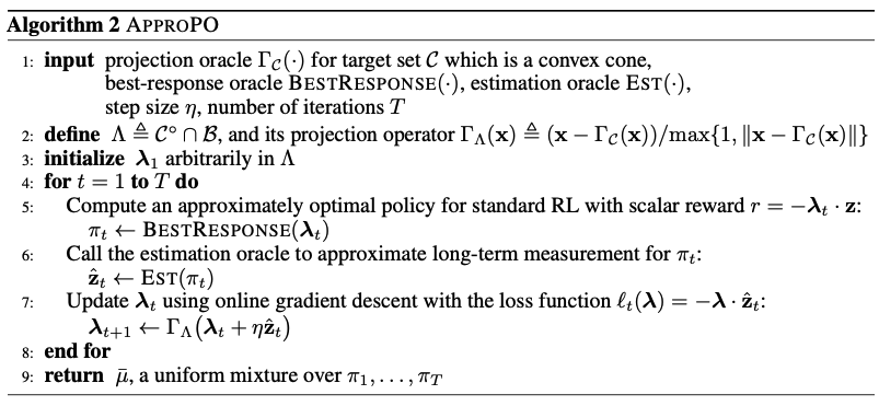
After $\mu$ -player returns the best $\mu$ , $\lambda$ -player can again return a new $\pmb{\lambda}$ based on $\bar{\pmb{z}}(\mu)$ . Then $\mu$ -player again returns the best policy learned on the scalar reward $-\pmb{\lambda}\cdot \bar{\pmb{z}}$ . The iterations go on for $T$ steps. Finally the algorithm would return a random mixture of $\mu$ from all iteration steps.

My concern is that this algorithm could not easily be extended to the batch learning context. Although the best response algorithm can always use an off-policy algorithm to learn $\pi$ without recollecting data, determining the optimal $\pmb{\lambda}$ needs to know $\bar{\pmb{z}}(\pi)$ , the estimation of $\pi$ on all dimensions of rewards. This would be super inaccurate using any off-policy evaluation method. There is also a question on how to serve the mixture of policies rather than just one single policy.

References

[1] Reinforcement Learning with Convex Constraints

Hash table revisited

I came across how Facebook implements Hash table from this post: https://engineering.fb.com/developer-tools/f14/. It introduces several techniques making modern hash tables more efficient.

The first technique is called chunking, which reduces the time for resolving hash collision. The idea is to map keys to a chunk (a block of slots) rather than a single slot then search within the chunk in parallel. Specifically, FB designates 14 slots in one chunk. I am not totally sure how, once a key is determined to belong to a chunk, a slot within the chunk is allocated for that key. For now I assume allocating a slot in a chunk is super fast, as indicated by the article that the search within the chunk is done through highly parallelizable vector instructions. In chunked hash tables, undesired cost would happen only in chunk overflow, i.e., if the chunk is full and a key needs to be relocated to another chunk. Similarly you can also call slot overflow in non-chunked hash tables for the scenario where a slot is full and a key needs to find another slot. The chance of seeing a chunk overflow (15 keys happen to belong to the same chunk) is much lower than seeing a slot overflow, hence chunking saves the time for resolving collision.

The second technique is called count-based tombstone. We can first revisit what is a tombstone in a classic hash table implementation. It refers to setting a slot to a special empty symbol when deleting an entry in a hash table. Tombstones are needed because the freed slots can hold new entries in the future but to reliably determine whether a to-be-inserted key exists we still need to probe beyond any tombstone slot encountered, as if that tombstone slot is not empty. We call the behavior “probe” as the process to search the next slot in the presence of key collision until we can determine whether the key exists or not. Probing can happen during either inserting or searching a key.

Tombstone is easily understood from an example:

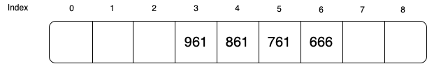
In the example, we use every key’s middle-digit as the primary hash function $h$ . We use the last-digit as the secondary hash function $i$ . When a key’s primary hash $j=h(k)$ is full, we probe the next position at $j=j-i(k)$ . The above hash table is generated by inserting 666, 761, 861 and 961 in order.

Suppose now we remove 761, followed by inserting 961 again. When 961 is probed first at index $j=h(961)=6$ , slot 6 is full. So next it probed $j=j-i(961)=6-1=5$ . Slot 5 is empty. However, if we had stopped at slot 5, we would wrongly assume 961 was not in the hash table. That’s why when we delete key 761, we need to mark slot 5 as a special empty symbol different than just a new blank slot.

Now let’s illustrate the idea of auxiliary-bit tombstones. For each slot, we use an extra bit to denote whether this slot is probed during insertion (recall probe can happen also in search). Then when we search a key, we can stop probing as soon as a 0 bit is encountered.

Auxiliary-bit tombstones can be illustrated in the following example. Suppose we generate a hash table by inserting 666, 761, 861, 333, 222, and 921 in order. Since 666 is probed during inserting 761 and 861, 761 is probed during inserting 861, and 222 is probed during inserting 921, the extra bit for 666, 761, and 222 is set to 1. After insertion, we remove key 861 and denote slot 4 as a tombstone.

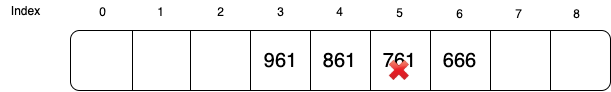
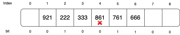
Now if we want to search if key 361 exists, it will start from index 6 (666). Without the extra bits, we will probe denoted until index 1 (the probe will pass slot 4 pretending it is a full slot). But with the extra bit, we will only need to probe until index 4. At index 4, we know no more key that sharing the same probe path has inserted beyond this point.

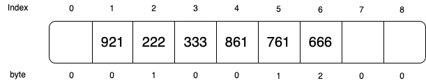
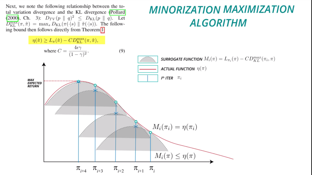
Facebook extends the auxiliary bits to auxiliary bytes which are used to count the insertion probes for each slot. Let’s create another hash table using the same data: 666, 761, 861, 333, 222, and 921 in order. The extra bytes are created as shown in the diagram. For example, since 666 is probed during inserting 761 and 861, its auxiliary byte stores 2.

If we remove 861, the auxiliary byte will be subtracted 1 on all the slots on its probe path:

Now, if want to search if key 361 exists, we will only need to probe until index 5 because slot 5’s auxiliary byte is 0. Comparing to just using auxiliary bits, we save more unnecessary probes.

The rest techniques are more C++ relevant, which I’ll skip.

EmbeddingBag from PyTorch

EmbeddingBag in PyTorch is a useful feature to consume sparse ids and produce embeddings.

Here is a minimal example. There are 4 ids’ embeddings, each of 3 dimensions. We have two data points, the first point has three ids (0, 1, 2) and the second point has the id (3). This is reflected in input and offsets variables: the i-th data point has the id from input[offset[i]] (inclusive) to input[offset[i+1]] (exclusive). Since we are using the “sum” mode, the first data point’s output would be the sum of the embeddings of ids (0, 1, 2), and the second data point’s output would be the embedding of id 3.

>>> embedding_sum = nn.EmbeddingBag(4, 3, mode='sum')
>>> embedding_sum.weight
Parameter containing:
tensor([[-0.9674, -2.3095, -0.2560],
        [ 0.0061, -0.4309, -0.7920],
        [-1.3457,  0.8978,  0.1271],
        [-1.8232,  0.6509, -1.2162]], requires_grad=True)
>>> input = torch.LongTensor([0,1,2,3])
>>> offsets = torch.LongTensor([0,3])
>>> embedding_sum(input, offsets)
tensor([[-2.3070, -1.8426, -0.9209],
        [-1.8232,  0.6509, -1.2162]], grad_fn=<EmbeddingBagBackward>)
>>> torch.sum(embedding_sum.weight[:3], dim=0)
tensor([-2.3070, -1.8426, -0.9209], grad_fn=<SumBackward1>)
>>> torch.sum(embedding_sum.weight[3:], dim=0)
tensor([-1.8232,  0.6509, -1.2162], grad_fn=<SumBackward1>)

Test with torch.multiprocessing and DataLoader

As we know PyTorch’s DataLoader is a great tool for speeding up data loading. Through my experience with trying DataLoader, I consolidated my understanding in Python multiprocessing.

Here is a didactic code snippet:

from torch.utils.data import DataLoader, Dataset
import torch
import time
import datetime
import torch.multiprocessing as mp
num_batches = 110

print("File init")

class DataClass:
    def __init__(self, x):
        self.x = x


class SleepDataset(Dataset):
    def __len__(self):
        return num_batches

    def __getitem__(self, idx):
        print(f"sleep on {idx}")
        time.sleep(5)
        print(f"finish sleep on {idx} at {datetime.datetime.now()}")
        return DataClass(torch.randn(5))


def collate_fn(batch):
    assert len(batch) == 1
    return batch[0]


def _set_seed(worker_id):
    torch.manual_seed(worker_id)
    torch.cuda.manual_seed(worker_id)


if __name__ == "__main__":
    mp.set_start_method("spawn")
    num_workers = mp.cpu_count() - 1
    print(f"num of workers {num_workers}")
    dataset = SleepDataset()
    dataloader = DataLoader(
        dataset,
        batch_size=1,
        shuffle=False,
        num_workers=num_workers,
        worker_init_fn=_set_seed,
        collate_fn=collate_fn,
    )

    dataloader = iter(dataloader)
    for i in range(1000):
        print(next(dataloader).x)

We have a Dataset called SleepDataset which is faked to be computationally expensive. We allow DataLoader to use all available processes (except the main process) to load the dataset. Python3 now has three ways to start processes: fork, spawn, and forkserver. I couldn’t find much online information regarding forkserver. But the difference between fork and spawn has been discussed a lot online: fork is only supported in Unix system. It creates a new process by copying the exact memory of the parent process into a new memory space and the child process can continue to execute from the forking point [3]. The system can still distinguish parent and child processes by process ids [1]. On the other hand, spawn creates new processes by initializing from executable images (files) rather than directly copying the memory from the parent process [2].

Based on these differences, if we let mp.set_start_method("spawn"), we find “File init” will be printed first at the main process then be printed every time a DataLoader process is created (110 times since num_batches = 110). If we let mp.set_start_method("fork"), we find “File init” will only be printed once. “forkserver” method behaves similarly to “spawn”, as we also see 110 times of “File init” being printed.

[1] https://qr.ae/TS6uaJ

[2] https://www.unix.com/unix-for-advanced-and-expert-users/178644-spawn-vs-fork.html

[3] https://www.python-course.eu/forking.php

Indexing data on GPU

This correspond a question I asked on Pytorch forum. When we want to use indexing to extract data which is already on GPU, should indexing arrays better be on GPU as well? The answer is yes. Here is the evidence:

I also created some other examples to show that if you are generating indexing arrays on the fly, they should be best created using torch.xxx(..., device=torch.device("cuda") rather than torch.xxx(...).

TRPO, PPO, Graph NN + RL

Writing this post to share my notes on Trust Region Policy Optimization [2], Proximal Policy Optimization [3], and some recent works leveraging graph neural networks on RL problems.

We start from the objective of TRPO. The expected return of a policy is $\eta(\pi)=\mathbb{E}_{s_0, a_0, \cdots}[\sum\limits_{t=0}^{\infty}\gamma^t r(s_t)]$ . The return of another policy $\hat{\pi}$ can be expressed as $\eta(\pi)$ and a relative difference term: $\eta(\hat{\pi})=\eta(\pi) + \sum\limits_s \rho_{\hat{\pi}}(s)\sum\limits_a \hat{\pi}(a|s) A_{\pi}(s,a)$ , where for any given $\pi$ , $\rho_{\pit}(s)=P(s_0) + \gamma P(s_1=s) + \gamma^2 P(s_2=s) + \cdots$ is called discounted state visitation frequency.

To facilitate the optimization process, the authors propose to replace $\rho_{\hat{\pi}}(s)$ with $\rho_{\pi}(s)$ . If the new policy $\hat{\pi}$ is close to $\pi$ , this approximation is not that bad since the discounted state visitation frequency shouldn’t change too much. Thus $\eta(\hat{\pi}) \approx L_{\pi}(\hat{\pi})=\eta(\pi) + \sum\limits_s \rho_{\pi}(s)\sum\limits_a \hat{\pi}(a|s)A_{\pi}(s,a)$ .

Using some theorem (See section 3 [2]) we can prove that $\eta(\hat{\pi}) \geq L_{\pi}(\hat{\pi})-C \cdot D^{max}_{KL}(\pi, \hat{\pi})$ , where $C=\frac{4\epsilon\gamma}{(1-\gamma)^2}$ , $\epsilon=max_{s,a}|A_{\pi}(s,a)|$ , and $D^{max}_{KL}(\pi, \hat{\pi})=\max_s D_{KL}(\pi(\cdot|s) \| \hat{\pi}(\cdot|s))$ . The inequality-equality becomes just equality if $\hat{\pi}=\pi$ . Therefore, $\arg\max_{\hat{\pi}}[L_{\pi}(\hat{\pi})-C\cdot D^{max}_{KL}(\pi, \hat{\pi})] \geq L_{\pi}(\pi)-C\cdot D^{max}_{KL}(\pi, \pi)=L_{\pi}(\pi)$ . 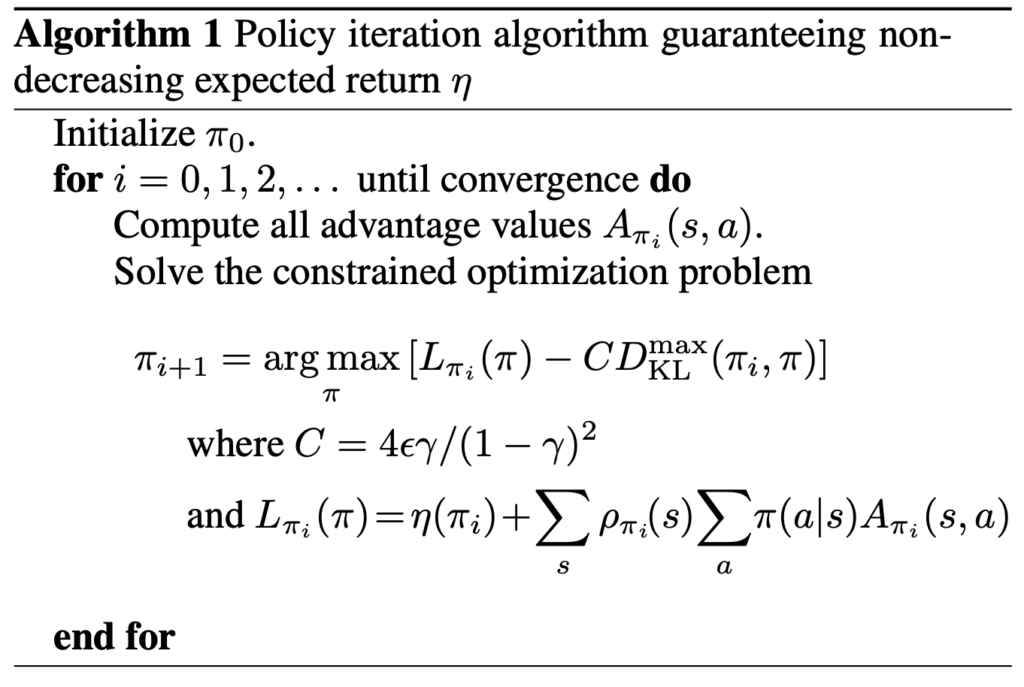Therefore, we can use algorithm 1 to monotonically improve $\pi$ .

The algorithm 1 can also be understood through the diagram below (from [10]), where we set $M_i(\pi)=L_{\pi_i}(\pi)-CD^{max}_{KL}(\pi_i, \pi)$ .

In practice, we parameterize a policy with $\theta$ , and we move the coefficient $C$ from the objective to a constraint (the paper argues this could improve the policy in larger steps), and finally we use the average KL divergence between two policies rather than $D^{max}_{KL}$ . Putting these practical treatments together, we get:

$\arg\max\limits_{\theta} L_{\pi_{\theta_{old}}}(\pi_{\theta})=\sum\limits_s \rho_{\pi_{\theta_{old}}}(s)\sum\limits_a \pi_\theta(a|s)A_{\pi_{\theta_{old}}}(s,a) \newline \text{subject to } \bar{D}^{\rho_{\pi_{\theta_{old}}}}_{KL}(\pi_{\theta_{old}}, \pi_{\theta})\leq \delta$

If changing the sum to expectation $\mathbb{E}_{s\sim \rho_{\theta_{old}}, a\sim \pi_{\theta_{old}}}$ , we will need some importance-sampling re-weighting. And in practice, we can estimate Q-values from trajectories more easily than estimating advantages because we would need exhaust all actions at each step to compute advantages. Thus the objective function using empirical samples eventually becomes:

$\arg\max\limits_{\theta} \mathbb{E}_{s\sim \rho_{\pi_{\theta_{old}}}, a\sim \pi_{\theta_{old}}} \big[\frac{\pi_{\theta}(a|s)}{\pi_{\theta_{old}}(a|s)} Q_{\pi_{\theta_{old}}}(s,a)\big] \newline \text{subject to } \mathbb{E}_{s\sim \rho_{\pi_{\theta_{old}}}} \big[D_{KL}(\pi_{\theta_{old}}(\cdot|s) \| \pi_{\theta}(\cdot|s))\big]\leq \delta$

Suppose the objective is $f(\theta)=\frac{\pi_{\theta}(s|a)}{\pi_{\theta_{old}}(a|s)} Q_{\pi_{\theta_{old}}}(s,a)$ . Using Taylor series expansion, we have $f(\theta) \approx f(\theta_{old}) + \nabla_\theta f(\theta)|_{\theta=\theta_{old}}(\theta-\theta_{old})=f(\theta_{old}) + g^T (\theta-\theta_{old})$ . $f(\theta_{old})$ can be seen as a constant and thus can be ignored during optimization.

And for the constraint, we can also use Taylor series expansion (this is a very common trick to convert KL divergence between two distributions into Taylor series expansion). Suppose $h(\theta)=D_{KL}(\pi_{\theta_{old}}(\cdot|s) \| \pi_{\theta}(\cdot|s))$ , then $h(\theta)\approx h(\theta_{old}) + \nabla_\theta h(\theta) |_{\theta=\theta_{old}} (\theta-\theta_{old})+\frac{1}{2}(\theta-\theta_{old})^T \nabla^2_\theta h(\theta)|_{\theta=\theta_{old}}(\theta-\theta_{old})$ . We know that $h(\theta_{old})=0$ because it is the KL divergence between the same distribution $\pi_{\theta_{old}}$ . We can also know that $\nabla_\theta h(\theta) |_{\theta=\theta_{old}}=0$ because the minimum of KL divergence is 0 and is reached when $\theta=\theta_{old}$ hence the derivative at $\theta_{old}$ must be 0.

Removing all constant and zero terms, and with two more notations $s=\theta-\theta_{old}$ and $H=\nabla^2_\theta h(\theta)|_{\theta=\theta_{old}}$ , we rewrite the objective function as well as the constraint:

$\arg\min\limits_{s} -g^T s \newline\text{ subject to } \frac{1}{2}s^T H s - \delta \leq 0$

Now the Lagrange Multiplier optimization kicks in. Intuitively, the direction to get to the next $\theta$ is on the direction that minimizes $-g^T s$ while stretching the constraint by the most extent (at the moment when the equality of the constraint holds). Denote the Lagrange Multiplier as $\lambda$ (a single scalar because we only have one constraint) and the auxiliary objective function as $\mathcal{L}(s, \lambda)=-g^T s + \lambda (\frac{1}{2}s^T H s - \delta)$ . From Karush-Kuhn-Tucker (KTT) conditions, we want to find a unique $\lambda^*$ and the local minimum solution $s^*$ such that:

$\nabla_s \mathcal{L}(s^*,\lambda^*)=0$
$\lambda^* \geq 0$
$\lambda^*\cdot (\frac{1}{2}s^T H s - \delta) = 0$
$\frac{1}{2}s^{*T} H s^* - \delta \leq 0$ (actually, the equality should hold because $s^*$ should be obtained at the border of the constraint, although I am not sure how to prove it. This means, as long as we find some non-negative $\lambda^*$ such that $\nabla_s \mathcal{L}(s^*,\lambda^*)=0$ , the first four conditions are satisfied.)
$\nabla^2_s \mathcal{L}(x^*, \lambda^*)$ is positive semi-definite. $\nabla^2_s \mathcal{L}(x^*, \lambda^*)$ is just $H$ times some constant term. And we know from the fact that: (1) $H$ is the Fisher information matrix because it is the Hessian of KL divergence [12]; (2) a Fisher information matrix is positive semi-definite [13].

Since we don’t have analytical solution for $\frac{1}{2}s^{*T} H s^* - \delta = 0$ , we can’t know $s^*$ easily. We can start from looking at $\nabla_s \mathcal{L}(s^*,\lambda^*)=-g + \lambda^* Hs^* = 0$ . Moving $-g$ to the right side, we have $\lambda^* H s^*=g$ . Here, both $s^*$ and $\lambda^*$ are unknown to us. But we know that $s^*=\lambda^{*-1}H^{-1}g$ . Therefore, $s^*$ must be in the direction of $H^{-1}g$ . How to compute $H^{-1}g$ ? If we just compute $H^{-1}$ as pure matrix inversion, we would need $O(n^3)$ time complexity where $n$ is width/height of $H$ . Instead, we can first obtain the solution $x$ of the equation $H x=g$ using Conjugate Gradient Method; $x$ will be exactly $H^{-1}g$ . We will spend one section below to introduce Conjugate Gradient method but for now just remember Conjugate Gradient method can compute $x$ much faster than $O(n^3)$ as in matrix inversion. Back to our focus: once we get $H^{-1}g$ , we will try to take the step size $\beta$ that makes the constraint equality hold: $\frac{1}{2} \beta x^T H \beta x - \delta=0$ . Thus the $\beta$ would be obtained at $\beta=\sqrt{(\frac{2\delta}{x^T H x})}$ . Therefore, $\theta = \theta_{old}+\beta x$ . This is exactly one iteration of TRPO update!

We now introduce what the conjugate gradient method is, which is used to find the update direction in TRPO.

Conjugate Gradient Method

My summary is primarily based on [6]. CG is an iterative, efficient method to solve $Ax=b$ , which is the solution of the quadratic form $argmin_x f(x)=argmin_x \frac{1}{2}x^TAx-b^Tx+c$ . The most straightforward way to solve $Ax=b$ is to compute $A^{-1}$ and let $x=A^{-1}b$ . However, computing $A^{-1}$ needs $O(n^3)$ time complexity by Gaussian elimination method, where $n$ is the width (or height) of $A$ .

If we can’t afford to compute $A^{-1}$ , the best bet is to rely on iterative methods. We list some notations used across iterative methods before we proceed. The error $e_i=x_i - x$ is the distance between the i-th solution $x_i$ and the real solution $x$ . The residual $r_i=-f'(x_i)=b-Ax_i$ indicates how far we are from $b$ .

Steepest gradient descent with line search works as follows. At solution $x_i$ , take a step on the direction of $r_i$ , and the step size is determined such that the arrival point after the step, which is $x_{i+1}$ , should have the smallest $f(x_{i+1})$ . This can also be understood as $r_{i+1}$ should be orthogonal to $r_i$ . The two pictures below help illustrate the idea:

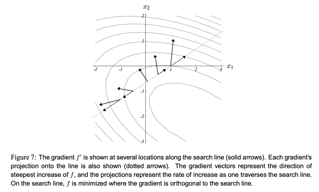
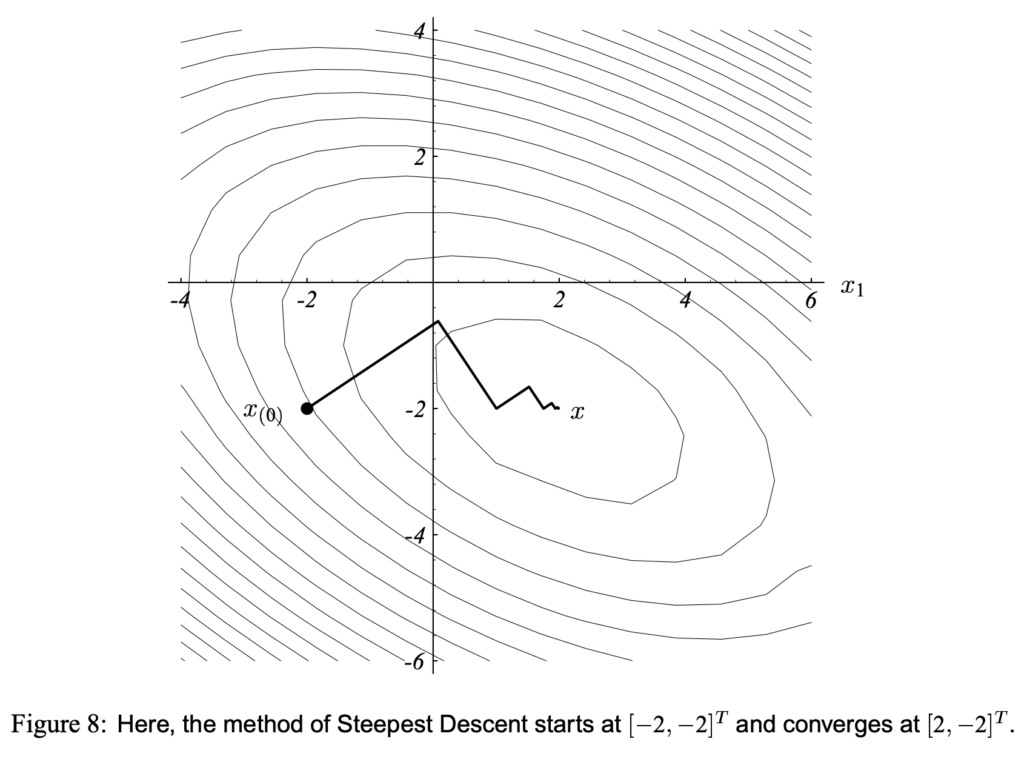
As you can see, the steepest gradient method often takes a zig-zag path to reach the sufficient proximity of the optimal solution. From theories (Section 6.2 in [6]), the number of steps it needs depends on the condition number of $A$ and the starting point $x_0$ . And from the intuition, the number of steps is no smaller than the number of bases of the solution space. The luckiest situation is that you pick $x_0$ which results to all orthogonal steepest gradients in the following steps. Such $x_0$ can also be thought to have $e_o$ parallel with any of the eigenvectors of $A$ :

The idea of conjugate direction methods (conjugate gradient is one of conjugate direction methods) is to enforce the iterations happen exactly $n$ times to reach the optimal solution, where, by our definition, $n$ is the width (or height) of $A$ and also the number of bases of the solution space.

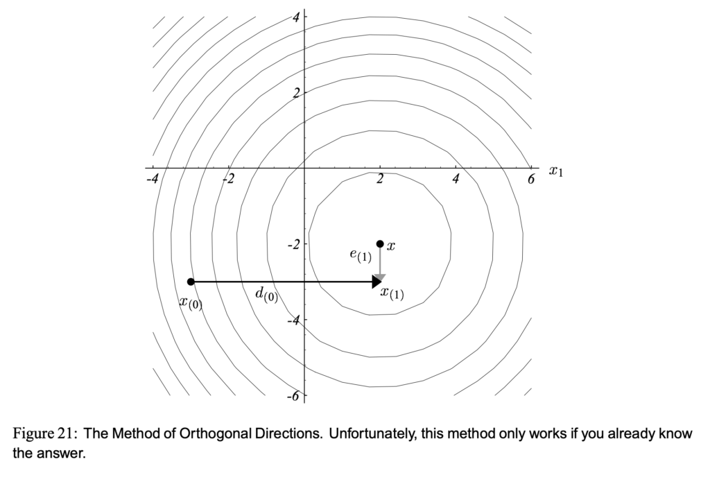
The procedure of conjugate direction methods starts from finding $d_0, d_1, \cdots, d_{n-1}$ search directions. If $d_0, d_1, \cdots, d_{n-1}$ can be orthogonal to each other, we can easily approach $x$ in $n$ steps, as in Figure 21. But theoretically we are not able to find such $n$ search directions. Instead, we can use Gram-Schmidt Conjugation and $u_0, u_1, \cdots, u_{n-1}$ linearly independent vectors to construct $n$ $A$ -orthogonal search directions. And it is provable that using $n$ $A$ -orthogonal search directions we can also approach $x$ in $n$ steps. However, for arbitrary $u_0, u_1, \cdots, u_{n-1}$ Gram-Schmidt Conjugation requires $O(n^2)$ space and $O(n^3)$ time complexity, which is a disadvantage in practice.

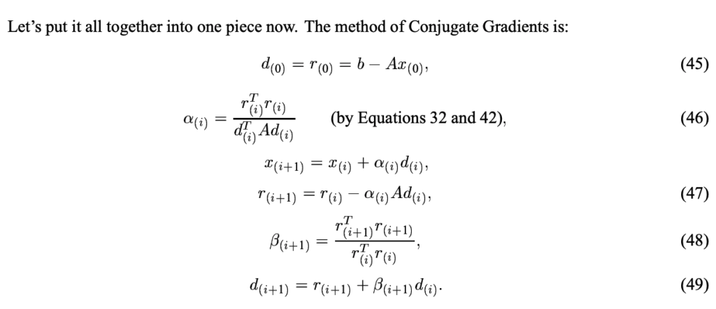
The method of conjugate gradients refers to the conjugate direction method when $u_0, u_1, \cdots, u_{n-1}$ are actually residuals $r_0, r_1, \cdots, r_{n-1}$ . Fortunately, it has a nice property that space complexity and time complexity can be reduced to $O(mn)$ , where $m$ is the number of nonzero entries of $A$ . Conjugate gradient can be summarized as follows:

Once you understand TRPO, PPO is much easier to be understood. PPO just simplifies the constrained optimization in TRPO to an unconstrained optimization problem. The main objective function of PPO is:

$L^{CLIP}\newline=CLIP\left(\mathbb{E}_{s\sim \rho_{\pi_{\theta_{old}}}, a\sim \pi_{\theta_{old}}} \left[\frac{\pi_{\theta}(a|s)}{\pi_{\theta_{old}}(a|s)} A_{\pi_{\theta_{old}}}(s,a)\right]\right)\newline=CLIP\left(\mathbb{E}_{s\sim \rho_{\pi_{\theta_{old}}}, a\sim \pi_{\theta_{old}}} \left[r(\theta)A_{\pi_{\theta_{old}}}(s,a)\right]\right)\newline=\mathbb{E}_{s\sim \rho_{\pi_{\theta_{old}}}, a\sim \pi_{\theta_{old}}} \left[min(r(\theta), clip(r(\theta), 1-\epsilon, 1+\epsilon)) \cdot A_{\pi_{\theta_{old}}}(s,a)\right]$

Let’s understand this clipped objective by some example. If $A_{\pi_{\theta_{old}}}(s,a)$ is positive, the model tries to increase $r(\theta)$ but no more than $1+\epsilon$ ; if $A_{\pi_{\theta_{old}}}(s,a)$ is negative, the model tries to decrease $r(\theta)$ but no less than $1-\epsilon$ . This way, the change of the policy is limited.

Now, let me examine the paper [5], because of which I started investigating TRPO and PPO. [5] models each joint in a robot in a locomotion task as a node in a graph. In graph learning, each node is represented as an embedding. At any given time step, the state feature can be summarized by all nodes’ embeddings. In [5], the policy network is learned through PPO.

[4] uses graph learning to model job scheduling graphs. But they use REINFORCE to learn their policy because their actions are defined as selecting one node out of all available nodes for scheduling.

Besides using graph learning to encode a graph into some feature representation, I’ve also seen people using tree-LSTM to encode tree-like graphs [14].

Reference

[1] Spinning Up doc about TRPO: https://spinningup.openai.com/en/latest/algorithms/trpo.html

[2] Trust Region Policy Optimization: https://arxiv.org/abs/1502.05477

[3] Proximal Policy Optimization Algorithms: https://arxiv.org/abs/1707.06347

[4] Learning Scheduling Algorithms for Data Processing Clusters: https://arxiv.org/abs/1810.01963

[5] NerveNet: Learning Structured Policy with Graph Neural Networks: https://openreview.net/pdf?id=S1sqHMZCb

[6] An Introduction to the Conjugate Gradient Method Without the Agonizing Pain: https://www.cs.cmu.edu/~quake-papers/painless-conjugate-gradient.pdf

[7] CS294-112 10/11/17: https://www.youtube.com/watch?v=ycCtmp4hcUs&feature=youtu.be&list=PLkFD6_40KJIznC9CDbVTjAF2oyt8_VAe3

[8] Towards Data Science PPO vs. TRPO: https://towardsdatascience.com/introduction-to-various-reinforcement-learning-algorithms-part-ii-trpo-ppo-87f2c5919bb9

[9] Efficiently Computing the Fisher Vector Product in TRPO: http://www.telesens.co/2018/06/09/efficiently-computing-the-fisher-vector-product-in-trpo/

[10] TRPO (Trust Region Policy Optimization) : In depth Research Paper Review: https://www.youtube.com/watch?v=CKaN5PgkSBc

[11] Optimization Overview: https://czxttkl.com/2016/02/22/optimization-overview/

[12] https://wiseodd.github.io/techblog/2018/03/14/natural-gradient/

[13] https://stats.stackexchange.com/questions/49942/why-is-the-fisher-information-matrix-positive-semidefinite

[14] Learning to Perform Local Rewriting for Combinatorial Optimization https://arxiv.org/abs/1810.00337

Dropbox Download

Notes on “Recommending What Video to Watch Next: A Multitask Ranking System”

Share some thoughts on this paper: Recommending What Video to Watch Next: A Multitask Ranking System [1]

The main contribution of this work is two parts: (1) a network architecture that learns on multiple objectives; (2) handles position bias in the same model

To first contribution is achieved by “soft” shared layers. So each objective does not necessarily use one set of expert parameters; instead it can use multiple sets of expert parameters controlled by a gating network:

The second contribution is to have a shallow network directly accounting for positions.

One thing that the paper is not clear about is how to finally use the multi-objective prediction. At the end of Section 4.2, it says:

we take the input of these multiple predictions, and output a combined score using a combination function in the form of weighted multiplication. The weights are manually tuned to achieve best performance on both user engagements and user satisfactions.

But I guess there might be some sweaty work needed to come to the optimal combination.

The final result looks pretty good, with improvement in all the metrics:

Since we are talking about position bias, I am interested to see some previous works in battling position bias, which is usually linked to contextual bandit works. The works in position bias and contextual bandit both battle with disproportionate data distribution. While position bias means certain logged samples are either over- or under-represented due to different levels of attention paid to different positions, contextual bandit models try to derive the optimal policy from the data distribution which is generated by sub-optimal policies thus is disproportionate to the data distribution by the optimal policy.

[2] introduces a fundamental framework for learning contextual bandit problems, coined as counterfactual risk minimization (CRM). A good mental model of contextual bandit models is that these models’ outputs are always stochastic and the output distribution keeps updated such that more probable actions should eventually correlate to the ones leading to higher returns.

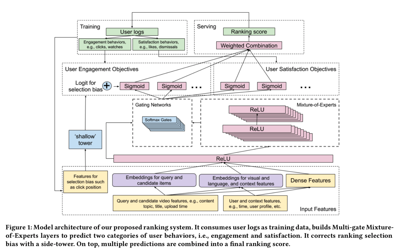
Note the objective used for batch w/bandit in Table 1. If you look at the paper [2], you’ll know that $\hat{R}^M(h)$ is some clipped version of importance sampling-based error:

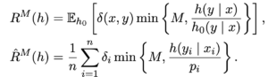
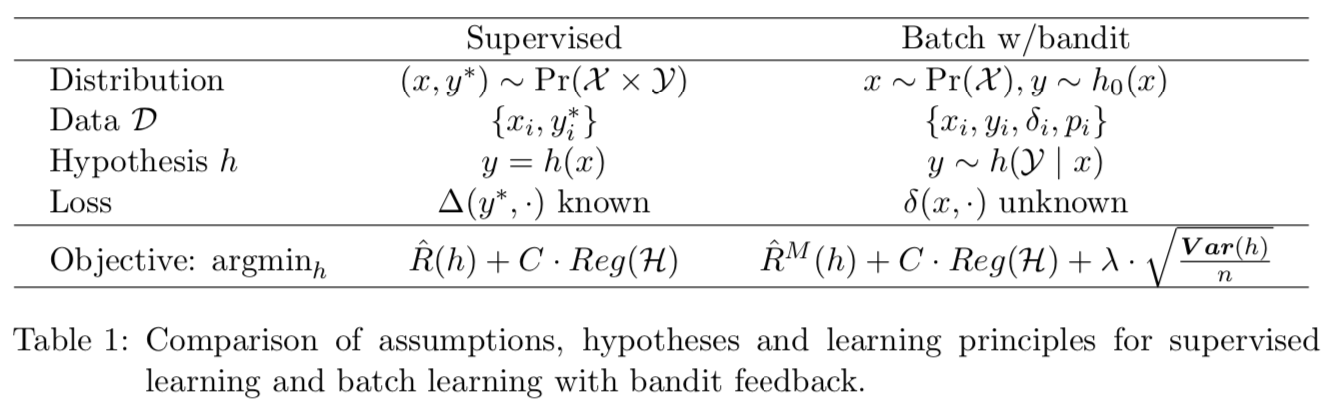
A typical loss function for contextual bandit models would be $\hat{R}^M(h)$ and [2]’s main contribution is to augment the loss function with $C\cdot Reg(\mathcal{H}) + \lambda \cdot \sqrt(Var(h)/n)$ (I need to verify if this sentence is correct). But as [2] suggested, the part $\lambda \cdot \sqrt(Var(h)/n)$ is said to “penalize the hypotheses with large variance during training using a data-dependant regularizer”.

Another sound previous work is [3]. The main idea is that a randomized dataset is used to estimate position bias. The intuition is simple: if you just randomize the order of a model’s ranking output, the click rate at each position would not be affected by any content placed on that content because content effects would be cancelled out by randomization. So the click rate at each position would only be related to the position itself, and that’s exactly position bias.

[4, 5] claims that you can account for position bias through Inverse Propensity Scores (IPS) when you evaluate a new ranking function based on implicit feedback (observable signals like clicks are implicit feedback, while the real user intent is explicit feedback but not always easily obtained). Intuitively, when we collect implicit feedback datasets like click logs, we need to account for observation bias because top positions certainly draw more feedbacks than bottom positions.

The learning-to-rank loss augmented by IPS is:

$\triangle_{IPS}(\mathbf{y} | \mathbf{x}_i, \bar{\mathbf{y}_i}, o_i)\newline=\sum\limits_{y:o_i(y)=1} \frac{rank(y|\mathbf{y})\cdot r_i(y)}{Q(o_i(y)=1|\mathbf{x}_i, \bar{\mathbf{y}_i}, r_i(y))}\newline=\sum\limits_{y:o_i(y)=1 \land r_i(y)=1}\frac{rank(y|\mathbf{y})}{Q(o_i(y)=1|\mathbf{x}_i, \bar{\mathbf{y}_i}, r_i(y))}$ ,

where $rank(y|\mathbf{y})$ is the rank of an item $y$ in the ranked list $\mathbf{y}$ by the new model, $\mathbf{\bar{y}_i}$ is the logged list, $Q(\cdot)$ denotes what is the probability of observing an item $y$ being clicked in the logged data. In the paper, the authors propose to express $Q(\cdot)$ as the probability of browsing the position of $y$ times the probability of clicking on $y$ .