I have been reading “Defensive Quantization: When Efficiency Meets Robustness” recently. Neural network quantization is a brand-new topic to me so I am writing some notes down for learning.
The first introduction I read is [1], from which I learn that the term “quantization” generally refers to reducing the memory usage of model weights by lowering representation precision. It could mean several similar concepts: (1) low precision: convert FP32 (floating point of 32 bits) to FP16, INT8, etc; (2) mixed precision, use FP16 for some weights while still keeping using FP32 for other weights (so that accuracy can be maintained); (3) exact quantization, basically using INT8 for all weights.
The next thing to understand is the basic of fixed-point and floating-point representation:
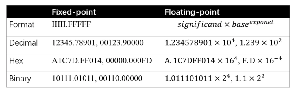
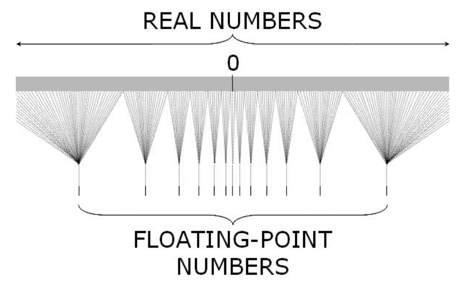
The fixed-point format saves the integer part and fractional part as separate numbers. Therefore, the precision between two consecutive fixed-point numbers is fixed. (For example, fixed-point numbers can be 123.456, 123.457, 123.458, …, with 0.001 between each two numbers.) The floating-point format saves a number as  so significand and exponent are saved as two separate numbers. Note that the precision between two consecutive floating-point numbers is not fixed but actually depends on exponents. For every exponent, the number of representable floating-point numbers is the same. But for a smaller exponent, the density of representable floating-point numbers is high; while for a larger exponent, the density is low. As a result, the closer a real value number is to 0, the more accurate it can be represented as a floating-point number. In practice, floating-point numbers are quite accurate and precise even with the largest exponent.
The procedure to quantize FP32 to INT8 is shown in Eqn.6~9 in [1]. In short, you need to find a scale and a reference point ( in the equations) to make sure every FP32 can fall into INT8’s value range
 ![[0, 255]](https://czxttkl.com/wp-content/ql-cache/quicklatex.com-d19efe2d99bac51355042c3a1c252da3_l3.png "Rendered by QuickLaTeX.com") .
.

Eqn. 6 ~ 9 only describes how to quantize weights but there is no guarantee that arithmetic operated on quantized weights would still fall into the quantized range. For example, there is an operator that adds two FP32 weights. While we can quantize the two weights into INT8, it is possible that the operator would result to overflow after adding the two quantized weights. Therefore, people have designed dedicated procedures to perform quantized arithmetic, such as multiplication, addition, subtraction, so on. See Eqn. 10~16 and 17~26 for the example of multiplication and addition, respectively.
While quantization is one way to reduce memory usage of models, compression is another alternative. [3] is one very famous work on compressing deep learning models.
Since I am an RL guy, I’d also like to introduce another work [4]. This work uses RL for model compression. They designed an MDP where the state is each layer’s features, action is compression ratio per layer (so the dimension of action is one and range is (0,1)); reward is model performance on the validation dataset, only evaluated at the last step of the MDP. The reward can also be tweaked to add resource constraint, such as latency. The take-away result is accuracy can be almost preserved while model size is compressed to a good ratio.
References
[1] Neural Network Quantization Introduction
[2] Defensive Quantization: When Efficiency Meets Robustness
[4] AMC: AutoML for Model Compression and Acceleration on Mobile Devices
[5] https://www.geeksforgeeks.org/floating-point-representation-digital-logic/