In this post, I am doing a brief code walkthrough for the code written in https://medium.com/emergent-future/simple-reinforcement-learning-with-tensorflow-part-8-asynchronous-actor-critic-agents-a3c-c88f72a5e9f2
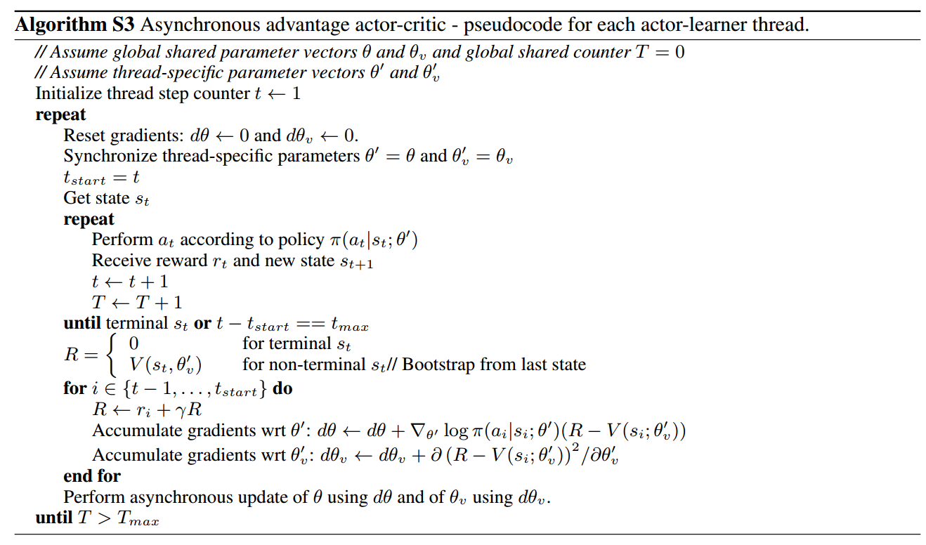
The code implements A3C algorithm (Asynchronous Methods for Deep Reinforcement Learning). It follows the pseudocode given in supplemental part in the paper:
The structure of this model is:
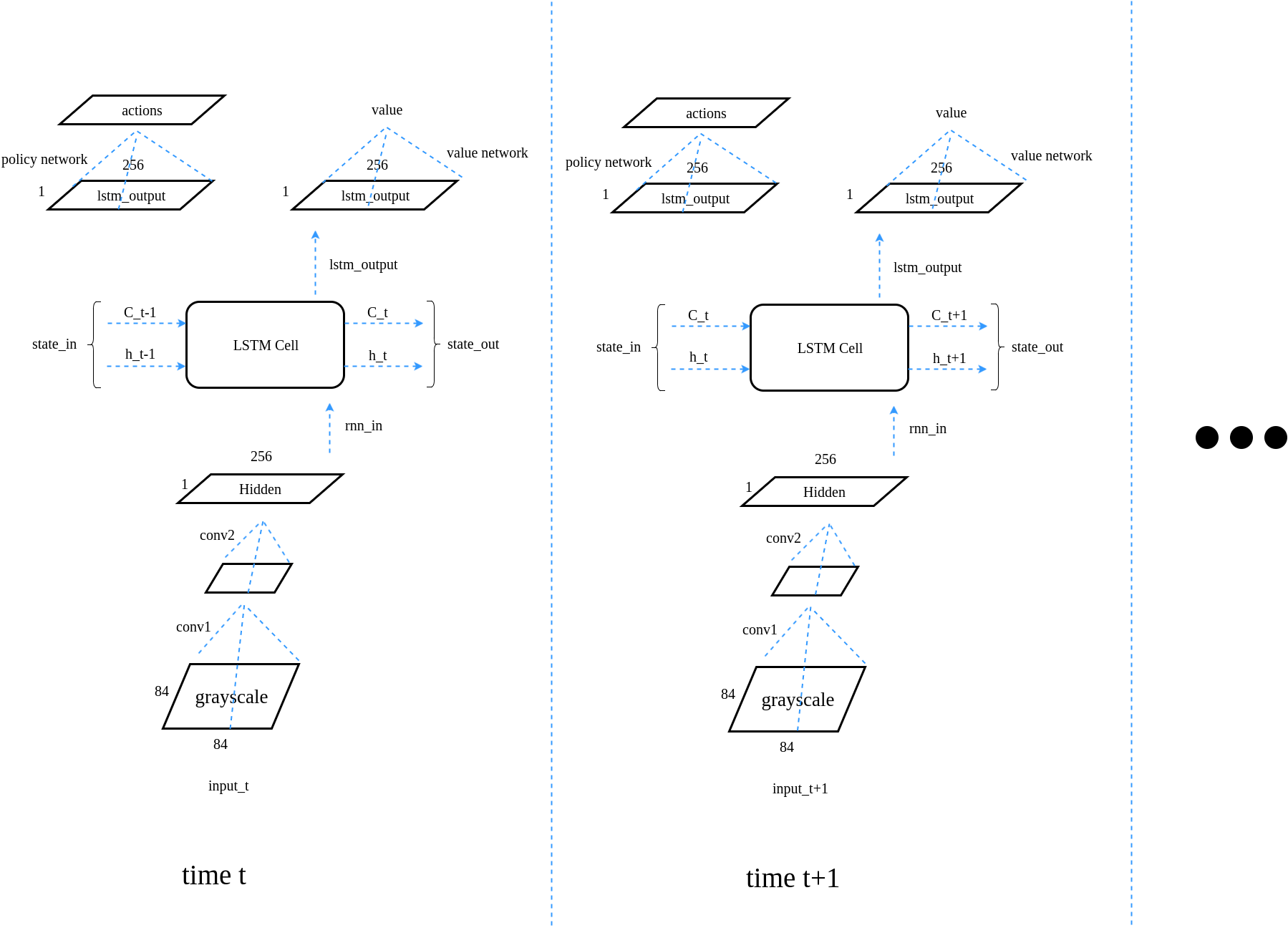
For LSTM structure detail, refer to http://colah.github.io/posts/2015-08-Understanding-LSTMs/. I am using the same notation in the model structure diagram as in the link.
Below is the code:
"""
Asynchronous Advantage Actor-Critic algorithm

See:
https://medium.com/emergent-future/simple-reinforcement-learning-with-tensorflow-part-8-asynchronous-actor-critic-agents-a3c-c88f72a5e9f2
https://arxiv.org/pdf/1602.01783.pdf
"""

import copy
import threading
import multiprocessing
import numpy as np
import matplotlib.pyplot as plt
import tensorflow as tf
import tensorflow.contrib.slim as slim
import scipy.signal
from helper import *
from vizdoom import *

from random import choice
from time import sleep
from time import time


# Copies one set of variables to another.
# Used to set worker network parameters to those of global network.
def update_target_graph(from_scope,to_scope):
    from_vars = tf.get_collection(tf.GraphKeys.TRAINABLE_VARIABLES, from_scope)
    to_vars = tf.get_collection(tf.GraphKeys.TRAINABLE_VARIABLES, to_scope)

    op_holder = []
    for from_var,to_var in zip(from_vars,to_vars):
        op_holder.append(to_var.assign(from_var))
    return op_holder

# Processes Doom screen image to produce cropped and resized image.
def process_frame(frame):
    s = frame[10:-10,30:-30]
    s = scipy.misc.imresize(s,[84,84])
    s = np.reshape(s,[np.prod(s.shape)]) / 255.0
    return s

# Discounting function used to calculate discounted returns.
def discount(x, gamma):
    return scipy.signal.lfilter([1], [1, -gamma], x[::-1], axis=0)[::-1]

#Used to initialize weights for policy and value output layers
def normalized_columns_initializer(std=1.0):
    def _initializer(shape, dtype=None, partition_info=None):
        out = np.random.randn(*shape).astype(np.float32)
        out *= std / np.sqrt(np.square(out).sum(axis=0, keepdims=True))
        return tf.constant(out)
    return _initializer


class AC_Network():
    def __init__(self, s_size, a_size, scope, trainer):
        with tf.variable_scope(scope):
            # Input and visual encoding layers
            self.inputs = tf.placeholder(shape=[None, s_size], dtype=tf.float32)
            self.imageIn = tf.reshape(self.inputs, shape=[-1, 84, 84, 1])
            self.conv1 = slim.conv2d(activation_fn=tf.nn.elu,
                                     inputs=self.imageIn, num_outputs=16,
                                     kernel_size=[8, 8], stride=[4, 4], padding='VALID')
            self.conv2 = slim.conv2d(activation_fn=tf.nn.elu,
                                     inputs=self.conv1, num_outputs=32,
                                     kernel_size=[4, 4], stride=[2, 2], padding='VALID')
            hidden = slim.fully_connected(slim.flatten(self.conv2), 256, activation_fn=tf.nn.elu)

            # Recurrent network for temporal dependencies
            lstm_cell = tf.contrib.rnn.BasicLSTMCell(256, state_is_tuple=True)
            self.lstm_cell_c_size = lstm_cell.state_size.c
            self.lstm_cell_h_size = lstm_cell.state_size.h
            c_init = np.zeros((1, lstm_cell.state_size.c), np.float32)
            h_init = np.zeros((1, lstm_cell.state_size.h), np.float32)
            self.state_init = [c_init, h_init]

            c_in = tf.placeholder(tf.float32, [1, lstm_cell.state_size.c])
            h_in = tf.placeholder(tf.float32, [1, lstm_cell.state_size.h])
            self.state_in = (c_in, h_in)
            rnn_in = tf.expand_dims(hidden, [0])
            step_size = tf.shape(self.imageIn)[:1]
            state_in = tf.contrib.rnn.LSTMStateTuple(c_in, h_in)
            lstm_outputs, lstm_state = tf.nn.dynamic_rnn(
                lstm_cell, rnn_in, initial_state=state_in, sequence_length=step_size,
                time_major=False)
            lstm_c, lstm_h = lstm_state
            self.state_out = (lstm_c[:1, :], lstm_h[:1, :])
            rnn_out = tf.reshape(lstm_outputs, [-1, 256])

            # Output layers for policy and value estimations
            self.policy = slim.fully_connected(rnn_out, a_size,
                                               activation_fn=tf.nn.softmax,
                                               weights_initializer=normalized_columns_initializer(0.01),
                                               biases_initializer=None)
            self.value = slim.fully_connected(rnn_out, 1,
                                              activation_fn=None,
                                              weights_initializer=normalized_columns_initializer(1.0),
                                              biases_initializer=None)

            # Only the worker network need ops for loss functions and gradient updating.
            if scope != 'global':
                self.actions = tf.placeholder(shape=[None], dtype=tf.int32)
                self.actions_onehot = tf.one_hot(self.actions, a_size, dtype=tf.float32)
                self.target_v = tf.placeholder(shape=[None], dtype=tf.float32)
                self.advantages = tf.placeholder(shape=[None], dtype=tf.float32)

                self.responsible_outputs = tf.reduce_sum(self.policy * self.actions_onehot, [1])

                # Loss functions
                self.value_loss = 0.5 * tf.reduce_sum(tf.square(self.target_v - tf.reshape(self.value, [-1])))
                self.entropy = - tf.reduce_sum(self.policy * tf.log(self.policy))
                self.policy_loss = -tf.reduce_sum(tf.log(self.responsible_outputs) * self.advantages)
                self.loss = 0.5 * self.value_loss + self.policy_loss - self.entropy * 0.01

                # Get gradients from local network using local losses
                local_vars = tf.get_collection(tf.GraphKeys.TRAINABLE_VARIABLES, scope)
                self.gradients = tf.gradients(self.loss, local_vars)
                self.var_norms = tf.global_norm(local_vars)
                grads, self.grad_norms = tf.clip_by_global_norm(self.gradients, 40.0)

                # Apply local gradients to global network
                global_vars = tf.get_collection(tf.GraphKeys.TRAINABLE_VARIABLES, 'global')
                self.apply_grads = trainer.apply_gradients(zip(grads, global_vars))

    def state_in_init(self):
        c_init = np.zeros((1, self.lstm_cell_c_size), np.float32)
        h_init = np.zeros((1, self.lstm_cell_h_size), np.float32)
        self.state_init = [c_init, h_init]


class Worker():
    def __init__(self, game, name, s_size, a_size, trainer, model_path, global_episodes):
        self.name = "worker_" + str(name)
        self.number = name
        self.model_path = model_path
        self.trainer = trainer
        self.global_episodes = global_episodes
        self.increment = self.global_episodes.assign_add(1)
        self.episode_rewards = []
        self.episode_lengths = []
        self.episode_mean_values = []
        self.summary_writer = tf.summary.FileWriter("train_" + str(self.number))

        # Create the local copy of the network and the tensorflow op to copy global paramters to local network
        self.local_AC = AC_Network(s_size, a_size, self.name, trainer)
        self.update_local_ops = update_target_graph('global', self.name)

        # The Below code is related to setting up the Doom environment
        game.set_doom_scenario_path("basic.wad")  # This corresponds to the simple task we will pose our agent
        game.set_doom_map("map01")
        game.set_screen_resolution(ScreenResolution.RES_160X120)
        game.set_screen_format(ScreenFormat.GRAY8)
        game.set_render_hud(False)
        game.set_render_crosshair(False)
        game.set_render_weapon(True)
        game.set_render_decals(False)
        game.set_render_particles(False)
        game.add_available_button(Button.MOVE_LEFT)
        game.add_available_button(Button.MOVE_RIGHT)
        game.add_available_button(Button.ATTACK)
        game.add_available_game_variable(GameVariable.AMMO2)
        game.add_available_game_variable(GameVariable.POSITION_X)
        game.add_available_game_variable(GameVariable.POSITION_Y)
        game.set_episode_timeout(300)
        game.set_episode_start_time(10)
        game.set_window_visible(False)
        game.set_sound_enabled(False)
        game.set_living_reward(-1)
        game.set_mode(Mode.PLAYER)
        game.init()
        self.actions = np.identity(a_size, dtype=bool).tolist()
        # End Doom set-up
        self.env = game

    def train(self, rollout, sess, gamma, bootstrap_value):
        rollout = np.array(rollout)
        observations = rollout[:, 0]
        actions = rollout[:, 1]
        rewards = rollout[:, 2]
        next_observations = rollout[:, 3]
        values = rollout[:, 5]

        # Here we take the rewards and values from the rollout, and use them to
        # generate the advantage and discounted returns.
        # The advantage function uses "Generalized Advantage Estimation"
        self.rewards_plus = np.asarray(rewards.tolist() + [bootstrap_value])
        discounted_rewards = discount(self.rewards_plus, gamma)[:-1]
        self.value_plus = np.asarray(values.tolist() + [bootstrap_value])
        advantages = rewards + gamma * self.value_plus[1:] - self.value_plus[:-1]
        advantages = discount(advantages, gamma)

        # Update the global network using gradients from loss
        # Generate network statistics to periodically save
        rnn_state = self.local_AC.state_init
        feed_dict = {self.local_AC.target_v: discounted_rewards,
                     self.local_AC.inputs: np.vstack(observations),
                     self.local_AC.actions: actions,
                     self.local_AC.advantages: advantages,
                     self.local_AC.state_in[0]: rnn_state[0],
                     self.local_AC.state_in[1]: rnn_state[1]}
        v_l, p_l, e_l, g_n, v_n, _ = sess.run([self.local_AC.value_loss,
                                               self.local_AC.policy_loss,
                                               self.local_AC.entropy,
                                               self.local_AC.grad_norms,
                                               self.local_AC.var_norms,
                                               self.local_AC.apply_grads],
                                              feed_dict=feed_dict)
        return v_l / len(rollout), p_l / len(rollout), e_l / len(rollout), g_n, v_n

    def work(self, max_episode_length, gamma, sess, coord, saver):
        episode_count = sess.run(self.global_episodes)
        total_steps = 0
        print("Starting worker " + str(self.number))
        with sess.as_default(), sess.graph.as_default():
            while not coord.should_stop():
                # copy global network parameter to self parameter
                sess.run(self.update_local_ops)
                # when a new episode starts, C_0 & h_0 of LSTM are reset to zero
                self.local_AC.state_in_init()
                episode_buffer = []
                episode_values = []
                episode_frames = []
                episode_reward = 0
                episode_step_count = 0
                d = False

                self.env.new_episode()
                s = self.env.get_state().screen_buffer
                episode_frames.append(s)
                s = process_frame(s)
                rnn_state = self.local_AC.state_init

                while self.env.is_episode_finished() == False:
                    # Take an action using probabilities from policy network output.
                    # after this step, a_dist shape (1,3), v shape (1,1),
                    # rnn_state: first array (C): (1, 256), second array (h): (1, 256)
                    a_dist, v, rnn_state = sess.run(
                        [self.local_AC.policy, self.local_AC.value, self.local_AC.state_out],
                        feed_dict={self.local_AC.inputs: [s],
                                   self.local_AC.state_in[0]: rnn_state[0],
                                   self.local_AC.state_in[1]: rnn_state[1]})
                    a = np.random.choice(a_dist[0], p=a_dist[0])
                    a = np.argmax(a_dist == a)     # return the best action index

                    # see http://vizdoom.cs.put.edu.pl/tutorial and
                    # https://github.com/mwydmuch/ViZDoom/blob/3bdb16935668aa42bb14cc38ac397b8954999cca/doc/DoomGame.md
                    # for reward description
                    # the agent gets rewards for each action which is -1 for each time tick,
                    # -6 if he shots but misses, and 100 if he kills the monster
                    r = self.env.make_action(self.actions[a]) / 100.0     # make_action returns reward

                    # In this example, the episode finishes after 300 tics or when the monster gets killed
                    # ref: http://www.cs.put.poznan.pl/visualdoomai/tutorial.html#basic - Game Runtime
                    d = self.env.is_episode_finished()
                    if d == False:
                        s1 = self.env.get_state().screen_buffer
                        episode_frames.append(s1)
                        s1 = process_frame(s1)
                    else:
                        s1 = s

                    episode_buffer.append([s, a, r, s1, d, v[0, 0]])
                    episode_values.append(v[0, 0])

                    episode_reward += r
                    s = s1
                    total_steps += 1
                    episode_step_count += 1

                    # If the episode hasn't ended, but the experience buffer is full, then we
                    # make an update step using that experience rollout.
                    if len(episode_buffer) == 30 and d != True and episode_step_count != max_episode_length - 1:
                        # Since we don't know what the true final return is, we "bootstrap" from our current
                        # value estimation.
                        v1 = sess.run(self.local_AC.value,
                                      feed_dict={self.local_AC.inputs: [s],
                                                 self.local_AC.state_in[0]: rnn_state[0],
                                                 self.local_AC.state_in[1]: rnn_state[1]})
                        v1 = v1[0, 0]
                        v_l, p_l, e_l, g_n, v_n = self.train(episode_buffer, sess, gamma, v1)
                        episode_buffer = []
                        sess.run(self.update_local_ops)
                        # original code does not update state_init:
                        # in train function, rnn_state is always set to self.state_init which are two zero numpy arrays
                        self.local_AC.state_init = copy.deepcopy(rnn_state)
                    if d == True:
                        break

                self.episode_rewards.append(episode_reward)
                self.episode_lengths.append(episode_step_count)
                self.episode_mean_values.append(np.mean(episode_values))

                # Update the network using the experience buffer at the end of the episode.
                if len(episode_buffer) != 0:
                    v_l, p_l, e_l, g_n, v_n = self.train(episode_buffer, sess, gamma, 0.0)

                # Periodically save gifs of episodes, model parameters, and summary statistics.
                if episode_count % 5 == 0 and episode_count != 0:
                    if self.name == 'worker_0' and episode_count % 25 == 0:
                        time_per_step = 0.05
                        images = np.array(episode_frames)
                        make_gif(images, './frames/image' + str(episode_count) + '.gif',
                                 duration=len(images) * time_per_step, true_image=True, salience=False)
                    if episode_count % 250 == 0 and self.name == 'worker_0':
                        saver.save(sess, self.model_path + '/model-' + str(episode_count) + '.cptk')
                        print("Saved Model")

                    mean_reward = np.mean(self.episode_rewards[-5:])
                    mean_length = np.mean(self.episode_lengths[-5:])
                    mean_value = np.mean(self.episode_mean_values[-5:])
                    summary = tf.Summary()
                    summary.value.add(tag='Perf/Reward', simple_value=float(mean_reward))
                    summary.value.add(tag='Perf/Length', simple_value=float(mean_length))
                    summary.value.add(tag='Perf/Value', simple_value=float(mean_value))
                    summary.value.add(tag='Losses/Value Loss', simple_value=float(v_l))
                    summary.value.add(tag='Losses/Policy Loss', simple_value=float(p_l))
                    summary.value.add(tag='Losses/Entropy', simple_value=float(e_l))
                    summary.value.add(tag='Losses/Grad Norm', simple_value=float(g_n))
                    summary.value.add(tag='Losses/Var Norm', simple_value=float(v_n))
                    self.summary_writer.add_summary(summary, episode_count)

                    self.summary_writer.flush()
                if self.name == 'worker_0':
                    sess.run(self.increment)
                episode_count += 1


max_episode_length = 300
gamma = .99 # discount rate for advantage estimation and reward discounting
s_size = 7056 # Observations are greyscale frames of 84 * 84 * 1
a_size = 3 # Agent can move Left, Right, or Fire
load_model = False
model_path = './model'

tf.reset_default_graph()

if not os.path.exists(model_path):
    os.makedirs(model_path)

# Create a directory to save episode playback gifs to
if not os.path.exists('./frames'):
    os.makedirs('./frames')

with tf.device("/cpu:0"):
    global_episodes = tf.Variable(0, dtype=tf.int32, name='global_episodes', trainable=False)
    trainer = tf.train.AdamOptimizer(learning_rate=1e-4)
    master_network = AC_Network(s_size, a_size, 'global', None)  # Generate global network
    num_workers = multiprocessing.cpu_count()  # Set workers ot number of available CPU threads
    workers = []
    # Create worker classes
    for i in range(num_workers):
        workers.append(Worker(DoomGame(), i, s_size, a_size, trainer, model_path, global_episodes))
    saver = tf.train.Saver(max_to_keep=5)

with tf.Session() as sess:
    coord = tf.train.Coordinator()
    if load_model == True:
        print('Loading Model...')
        ckpt = tf.train.get_checkpoint_state(model_path)
        saver.restore(sess, ckpt.model_checkpoint_path)
    else:
        sess.run(tf.global_variables_initializer())

    # This is where the asynchronous magic happens.
    # Start the "work" process for each worker in a separate threat.
    worker_threads = []
    for worker in workers:
        worker_work = lambda: worker.work(max_episode_length, gamma, sess, coord, saver)
        t = threading.Thread(target=(worker_work))
        t.start()
        sleep(0.5)
        worker_threads.append(t)
    coord.join(worker_threads)
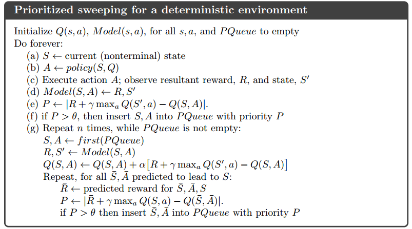
Note that Worker.train implements the loop $latex for \; i \in \{t-1, \cdots,t_{start}\}$ in the pseudocode.


 , where each
  is one regression tree’s output and
  are the parameters of that tree. Generally speaking, each regression tree has K-terminal nodes. Hence
  , which are the K feature subspaces that divide data, and
  , which are the predicted outputs of data belonging to
 are iteratively learned to fit to the training data:
 to initial guess
 , we learn optimal feature space divisions
 (leaf) is deterministically fixed as:
 . (If using this criteria,
  . The loss function
  is least square loss. Each regression tree is only a decision stump.
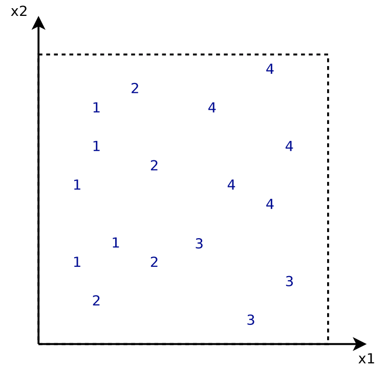
 is the simplest predictor that predicts a constant value minimizing the error for all training data.
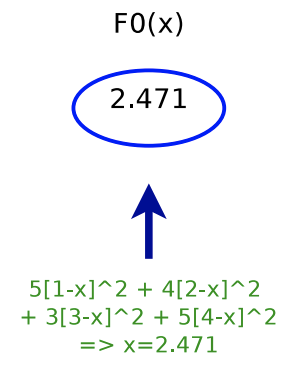
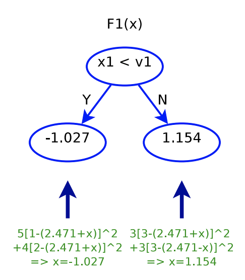
 , we start to build
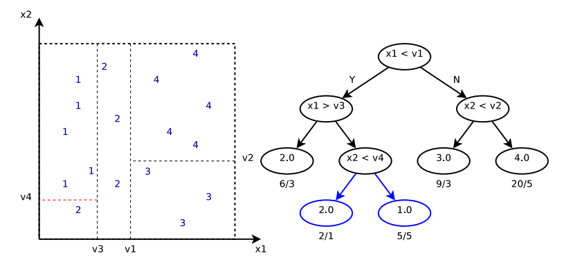
  . The cut
  is determined by some criterion not mentioned. But assuming that
  :
:
 . In other words, for
  , the predicted value will be 1.444; for
  , the predicted value will be 3.625.
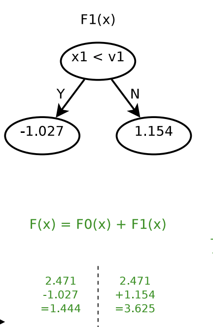
 will be similar: finding a cut
  , and then determine
  as in step 3.
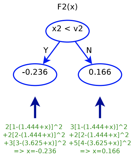
 , that is, we are fitting the residual of what previous trees are not able to predict. Below is the plot showing each data point’s original label and its updated label before fitting
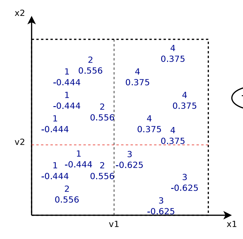
 is a square loss function. When fitting the
  -th tree, we are fitting the tree to the residual
  . Interestingly,
  . That’s why MART is also called Gradient Boosted Decision Tree because that each tree fits the gradient of the loss.

 and
and  . As long as we know
  and
and  , we can learn the best
  , then
  and
and  . Thus, the objective function becomes:
 . That’s why in the above fitting process, it seems like we are fitting each new tree to the residual between the real label and previous trees’ output. In another equivalent perspective, we are fitting each new tree to the gradient
  .
. is
is ![L(y_i, p_i)=- [y_i \log (p_i) + (1-y_i) \log (1-p_i)]](https://czxttkl.com/wp-content/ql-cache/quicklatex.com-e6faa5e549756e8e5ea8b26785a666f4_l3.png "Rendered by QuickLaTeX.com") , where
, where  is the predicted probability
  . The regression trees’ output is used to fit the logit of
 , then we have:
  See [11])
 (See [12])
 and
and  .
.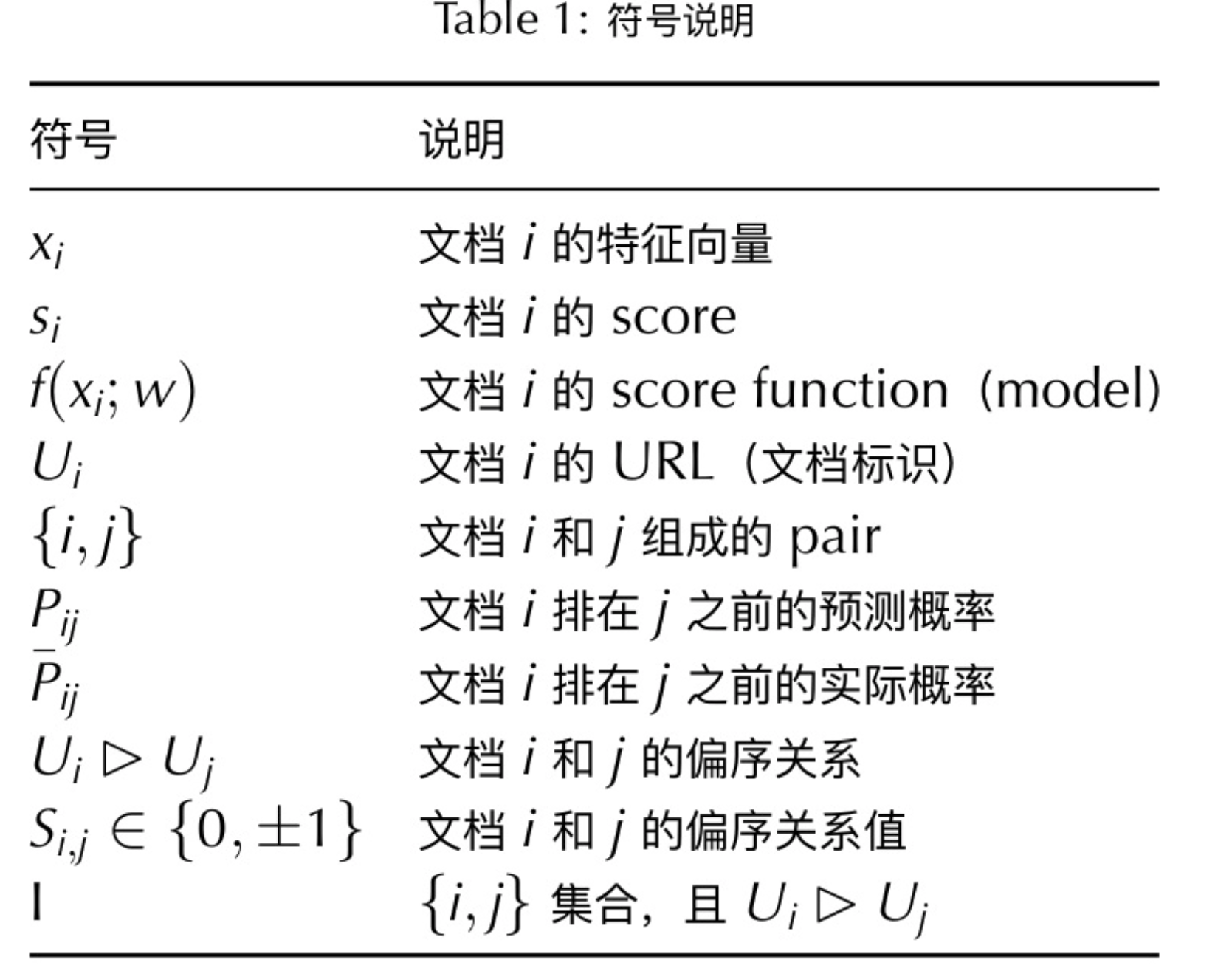

 ,
,  ; if
; if  . The intuition of this cost function is that the more consistent the relative order between
  and
and  is with
  , the smaller
  will be.
 , the cost function
  as example):
 , where
  . (This is from Eqn. 3 in [7].)
 is derived from a pair of URLs
  and
and  . For each document, we can aggregate to
  by taking into account of all its interaction with other documents:

 (
( , i.e., an increase of
  assuming
  . According to the update rule
  , immediately we know that
  or
or  , the scale of
  . On the other hand, if
  , that is, the current calculated scores are inconsistent with the label,
  will become relatively large (
 1).
1). 
 is the change after swapping
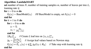
 is actually doing gradient ascent. Recall that in <1. MART> section the objective that each MART tree optimizes for is:
 corresponds to
  and
and  corresponds to
  .
.

 for any state-action pair, either by recording (“memorizing”) exact values in a tabular or learning a function to approximate it. Under
  -greedy, the action to be selected at a state will therefore be
  but there is also a small constant chance
  , where
  is the policy function’s parameters.
 , where
  is performance measure with respect to the policy weights.
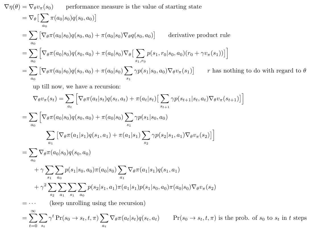
 . It can also be seen as an expectation of
  over the probability distribution of landing on
  in
in  steps. Please note for any fixed
  . Therefore, we can rewrite the above last expression as an expectation form:
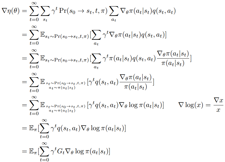
 .
.  is an unbiased estimator of
  in the last two steps since we do not have estimation for
  to replace
  , meaning that the sequence
  are generated following the policy
  and the transition probability
  . Sometimes we can also write
  because the policy
  is parameterized by
  . In other words,
 ![\nabla \eta(\theta) = \mathbb{E}_{s_{0:T}, a_{0:T}}[\sum\limits_{t=0}^T \gamma^t G_t \nabla_\theta \log \pi(a_t|s_t)] &s=2](https://czxttkl.com/wp-content/ql-cache/quicklatex.com-093ef803c0ca0df70cae9b9ecec84de5_l3.png "Rendered by QuickLaTeX.com")
 :
:
 , a function of
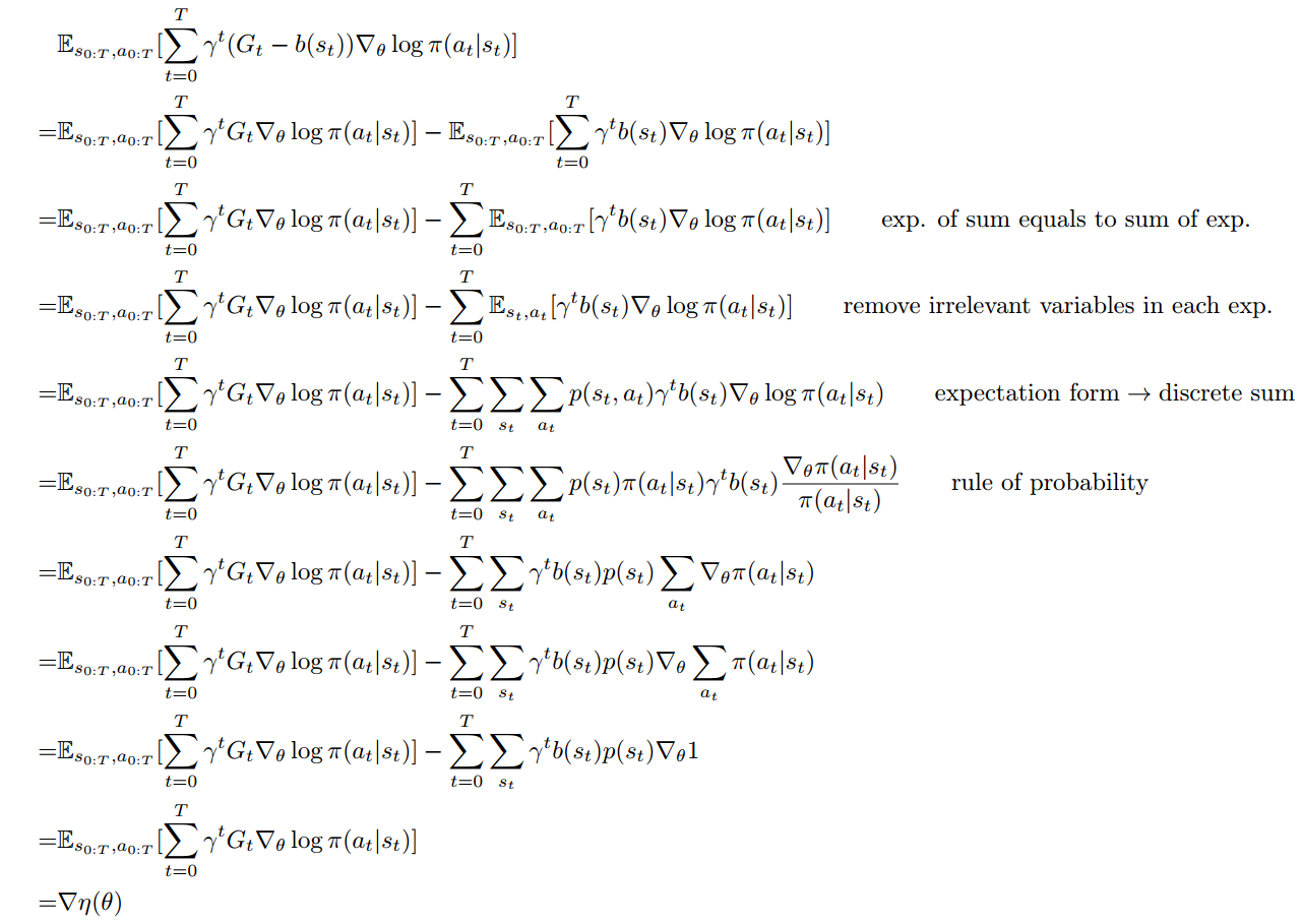
![\mathbb{E}_{s_{0:T}, a_{0:T}} [\sum\limits_{t=0}^T \gamma^t (G_t - b(s_t)) \nabla_\theta \log \pi (a_t|s_t)]](https://czxttkl.com/wp-content/ql-cache/quicklatex.com-8d586d2f867e3a9f19be27fbca1afe2b_l3.png "Rendered by QuickLaTeX.com") is an unbiased estimate of
is an unbiased estimate of  . Otherwise
 ![\mathbb{E}_{s_{0:T}, a_{0:T}}[\sum\limits_{t=0}^T \gamma^t b(s_t) \nabla_\theta \log \pi (a_t | s_t)]](https://czxttkl.com/wp-content/ql-cache/quicklatex.com-39cb9ee96a8a70267a3c0f0de4ba410e_l3.png "Rendered by QuickLaTeX.com") is not zero.
is not zero.![Var[ \sum\limits_{t=0}^T \gamma^t G_t \nabla_\theta \log \pi(a_t | s_t)]](https://czxttkl.com/wp-content/ql-cache/quicklatex.com-00b7d15eb73cf2b088fdad5a69ff16ac_l3.png "Rendered by QuickLaTeX.com") .
.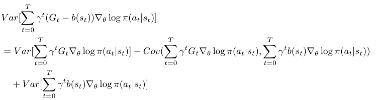
 has large enough covariance with
  to outweigh its own variance, then the variance is reduced. Unrealistically, if
  , then variance will be zero, although this is impossible because
  with parameter
![\mathbb{E}[G_t|S_t, A_t]=q_\pi(s_t, a_t)](https://czxttkl.com/wp-content/ql-cache/quicklatex.com-d172bdd4b1e22f48ae494f1aa7a44c42_l3.png "Rendered by QuickLaTeX.com") . However,
. However,  , where each reward can be seen as a random variable [13]. An alternative estimator of
  which has lower variance but higher bias is to use “bootstrapping”, i.e., use a parameterized value function
  plus the next immediate reward to approximate
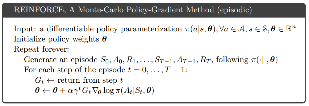
  . The one-step actor-critic algorithm is described as follows [1]:
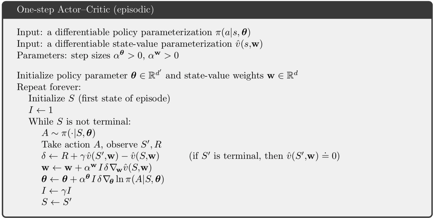
 in the gradient update depends on
  . The specific one-step actor-critic algorithm we just described is also an on-policy algorithm because
  depends on the next state
  which is the result of applying
  . There also exists off-policy actor-critics, see an overview of on-policy and off-policy policy gradient methods at [14].
 and
and  , in an un-discounted reward problem to help estimate
 ![g:=\nabla_\theta \mathbb{E}[\sum_{t=0}^\infty] r_t](https://czxttkl.com/wp-content/ql-cache/quicklatex.com-675a43e0384f3db1622065126706063a_l3.png "Rendered by QuickLaTeX.com") with little introduced bias and reduced variance. (Note that how discounted reward problems can be transformed into an un-discounted problem: “But the discounted problem (maximizing
with little introduced bias and reduced variance. (Note that how discounted reward problems can be transformed into an un-discounted problem: “But the discounted problem (maximizing  can be handled as an instance of the undiscounted problem in which we absorb the discount factor into the reward function, making it time-dependent.”)
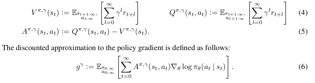
 is a biased estimator of
  but as they claim previous works have studied to “reduce variance by downweighting rewards corresponding to delayed effects, at the cost of introducing bias”.
 which is called
  .
.

 and
and  are functions with input as the whole trajectory
  . Similarly, think
  as a function with the input as the former part of the trajectory
  .
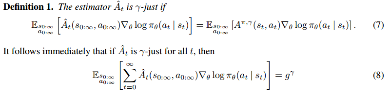
. where for all
  , then:
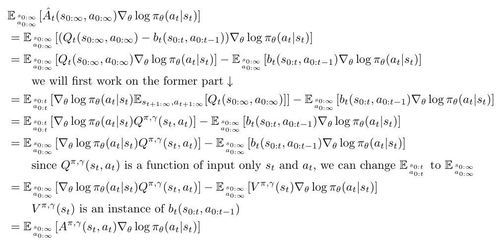
 . Only when we know
  is
is 
 is a biased estimator of
  (equation 11, 12, 13, 14, 15, and 16), then we might get a low bias, low variance estimator, which is called
  .
.
 is
is ![E_{s_{0:\infty}, a_{0:\infty}}[V(s_t) \nabla_\theta \log \pi_\theta (a_t | s_t) ] = 0](https://czxttkl.com/wp-content/ql-cache/quicklatex.com-aa027001db3204456c33147caf9929e0_l3.png "Rendered by QuickLaTeX.com") ). However
). However  is believed (I don’t know how to prove that) to have high variance due to the long sum of rewards. On the other extreme end,
  has low variance but since we are estimating the value function
  would make a trade-off between variance and bias.
![\begin{align*} \nabla \eta(\theta) &= \nabla_\theta v_{\pi} (s_0) \quad \quad \text{performance measure is the value of starting state} \\ &= \nabla_\theta \big[ \sum\limits_{a_0} \pi(a_0|s_0) q(s_0,a_0) \big] \\ &=\sum\limits_{a_0} \big[ \nabla_\theta \pi(a_0|s_0) q(s_0, a_0) + \pi(a_0|s_0) \nabla_\theta q(s_0, a_0) \big] \quad \quad \text{derivative product rule} \\ &= \sum\limits_{a_0} \Big[ \nabla_\theta \pi(a_0|s_0) q(s_0, a_0) + \pi(a_0|s_0) \nabla_\theta \big[ \sum\limits_{s_1,r_0} p(s_1, r_0 |s_0,a_0)(r_0 + \gamma v_\pi(s_1)) \big] \Big] \\ &= \sum\limits_{a_0} \big[ \nabla_\theta \pi (a_0 | s_0) q(s_0, a_0) + \pi(a_0 | s_0) \sum\limits_{s_1} \gamma p(s_1| s_0, a_0) \nabla_\theta v_{\pi}(s_1) \big] \qquad r \text{ has nothing to do with regard to } \theta \\ & \qquad \text{up till now, we have a recursion:} \\ & \qquad \nabla_\theta v_\pi(s_t)= \sum\limits_{a_t} \Big[ \nabla_\theta \pi(a_t|s_t) q(s_t, a_t) + \pi(a_t|s_t) \big[ \sum\limits_{s_{t+1}} \gamma p(s_{t+1}|s_t,a_t) \nabla_\theta v_\pi(s_{t+1}) \big] \Big] \\ &=\sum\limits_{a_0} \Big[ \nabla_\theta \pi (a_0 | s_0) q(s_0, a_0) + \pi(a_0 | s_0) \sum\limits_{s_1} \gamma p(s_1| s_0, a_0) \\ & \qquad \qquad \sum\limits_{a_1} \big[ \nabla_\theta \pi(a_1 | s_1)q(s_1, a_1) + \pi(a_1 | s_1)\sum\limits_{s_2} \gamma p(s_2|s_1, a_1) \nabla_\theta v_{\pi} (s_2) \big] \Big] \\ &=\sum\limits_{a_0} \nabla_\theta \pi (a_0 | s_0) q(s_0, a_0) \\ & \qquad + \gamma \sum\limits_{s_1} \sum\limits_{a_0} p(s_1| s_0, a_0) \pi(a_0 | s_0) \sum\limits_{a_1} \nabla_\theta \pi(a_1 | s_1)q(s_1, a_1) \\ & \qquad + \gamma^2 \sum\limits_{s_2} \sum\limits_{a_1} \sum\limits_{s_1} \sum\limits_{a_0} p(s_2|s_1, a_1) \pi(a_1 | s_1) p(s_1| s_0, a_0) \pi(a_0 | s_0) \nabla_\theta v_{\pi} (s_2) \\ &= \cdots \qquad \text{(keep unrolling using the recursion)}\\ &= \sum\limits_{t=0}^\infty \sum\limits_{s_t} \gamma^t \Pr(s_0 \rightarrow s_t, t, \pi) \sum\limits_{a_t} \nabla_\theta \pi(a_t | s_t) q(s_t, a_t) \qquad \Pr(s_0 \rightarrow s_t, t, \pi) \text{ is the prob. of } s_0 \text{ to } s_t \text{ in } t \text{ steps} \end{align*}](https://czxttkl.com/wp-content/ql-cache/quicklatex.com-8ade309cbfbab77fb5d741c4ea3a7df6_l3.png "Rendered by QuickLaTeX.com")
![\begin{align*} \nabla \eta(\theta) &= \sum\limits_{t=0}^\infty \sum\limits_{s_t} \gamma^t \Pr(s_0 \rightarrow s_t, t, \pi) \sum\limits_{a_t} \nabla_\theta \pi(a_t | s_t) q(s_t, a_t) \\ &=\sum\limits_{t=0}^\infty \mathbb{E}_{s_t \sim \Pr(s_0 \rightarrow s_t, t, \pi)}[\sum\limits_{a_t} \gamma^t \nabla_\theta \pi(a_t | s_t) q(s_t, a_t) ] \\ &=\sum\limits_{t=0}^\infty \mathbb{E}_{s_t \sim \Pr(s_0 \rightarrow s_t, t, \pi)} [\sum\limits_{a_t} \gamma^t \pi(a_t | s_t) q(s_t, a_t) \frac{\nabla_\theta \pi(a_t | s_t)}{\pi(a_t | s_t)} ] \\ &=\sum\limits_{t=0}^\infty \mathbb{E}_{s_t \sim \Pr(s_0 \rightarrow s_t, t, \pi) \atop a_t \sim \pi(a_t | s_t) \quad}[ \gamma^t q(s_t, a_t) \frac{\nabla_\theta \pi(a_t | s_t)}{\pi(a_t | s_t)}] \\ &=\sum\limits_{t=0}^\infty \mathbb{E}_{s_t \sim \Pr(s_0 \rightarrow s_t, t, \pi) \atop a_t \sim \pi(a_t | s_t) \quad}[ \gamma^t q(s_t, a_t) \nabla_\theta \log \pi(a_t | s_t)] \qquad \nabla \log(x) = \frac{\nabla x}{x} \\ &=\mathbb{E}_{\pi}[ \sum\limits_{t=0}^\infty \gamma^t q(s_t, a_t) \nabla_\theta \log \pi(a_t | s_t)] \\ &=\mathbb{E}_{\pi}[ \sum\limits_{t=0}^\infty \gamma^t G_t \nabla_\theta \log \pi(a_t | s_t)] \end{align*}](https://czxttkl.com/wp-content/ql-cache/quicklatex.com-d532fc2a9f8b3c450bf990553854353e_l3.png "Rendered by QuickLaTeX.com")
![\begin{align*} &\mathbb{E}_{s_{0:T}, a_{0:T}} [ \sum\limits_{t=0}^T \gamma^t (G_t - b(s_t)) \nabla_\theta \log \pi(a_t | s_t)] \\ =& \mathbb{E}_{s_{0:T}, a_{0:T}} [ \sum\limits_{t=0}^T \gamma^t G_t \nabla_\theta \log \pi(a_t | s_t)] - \mathbb{E}_{s_{0:T}, a_{0:T}}[ \sum\limits_{t=0}^T \gamma^t b(s_t) \nabla_\theta \log \pi (a_t | s_t) ] \\ =& \mathbb{E}_{s_{0:T}, a_{0:T}} [ \sum\limits_{t=0}^T \gamma^t G_t \nabla_\theta \log \pi(a_t | s_t)] - \sum\limits_{t=0}^T \mathbb{E}_{s_{0:T}, a_{0:T}}[ \gamma^t b(s_t) \nabla_\theta \log \pi (a_t | s_t) ] \qquad \text{exp. of sum equals to sum of exp.}\\ =& \mathbb{E}_{s_{0:T}, a_{0:T}} [ \sum\limits_{t=0}^T \gamma^t G_t \nabla_\theta \log \pi(a_t | s_t)] - \sum\limits_{t=0}^T \mathbb{E}_{s_{t}, a_{t}}[ \gamma^t b(s_t) \nabla_\theta \log \pi (a_t | s_t) ] \qquad \text{remove irrelevant variables in each exp.}\\ =& \mathbb{E}_{s_{0:T}, a_{0:T}} [ \sum\limits_{t=0}^T \gamma^t G_t \nabla_\theta \log \pi(a_t | s_t)] - \sum\limits_{t=0}^T \sum\limits_{s_{t}} \sum\limits_{a_{t}} p(s_t, a_t) \gamma^t b(s_t) \nabla_\theta \log \pi (a_t | s_t) \qquad \text{expectation form} \rightarrow \text{discrete sum} \\ =& \mathbb{E}_{s_{0:T}, a_{0:T}} [ \sum\limits_{t=0}^T \gamma^t G_t \nabla_\theta \log \pi(a_t | s_t)] - \sum\limits_{t=0}^T \sum\limits_{s_{t}} \sum\limits_{a_{t}} p(s_t) \pi(a_t|s_t) \gamma^t b(s_t) \frac{\nabla_\theta \pi (a_t | s_t)}{\pi(a_t | s_t) } \qquad \text{rule of probability} \\ =& \mathbb{E}_{s_{0:T}, a_{0:T}} [ \sum\limits_{t=0}^T \gamma^t G_t \nabla_\theta \log \pi(a_t | s_t)] - \sum\limits_{t=0}^T \sum\limits_{s_{t}} \gamma^t b(s_t) p(s_t) \sum\limits_{a_{t}} \nabla_\theta \pi (a_t | s_t) \\ =& \mathbb{E}_{s_{0:T}, a_{0:T}} [ \sum\limits_{t=0}^T \gamma^t G_t \nabla_\theta \log \pi(a_t | s_t)] - \sum\limits_{t=0}^T \sum\limits_{s_{t}} \gamma^t b(s_t) p(s_t) \nabla_\theta \sum\limits_{a_{t}} \pi (a_t | s_t) \\ =& \mathbb{E}_{s_{0:T}, a_{0:T}} [ \sum\limits_{t=0}^T \gamma^t G_t \nabla_\theta \log \pi(a_t | s_t)] - \sum\limits_{t=0}^T \sum\limits_{s_{t}} \gamma^t b(s_t) p(s_t) \nabla_\theta 1 \\ =& \mathbb{E}_{s_{0:T}, a_{0:T}} [ \sum\limits_{t=0}^T \gamma^t G_t \nabla_\theta \log \pi(a_t | s_t)] \\ =& \nabla \eta(\theta) \end{align*}](https://czxttkl.com/wp-content/ql-cache/quicklatex.com-b260de314aa5bf15c7507b755c32d260_l3.png "Rendered by QuickLaTeX.com")
![\begin{align*} &\mathbb{E}_{s_{0:\infty} \atop a_{0:\infty}} [\hat{A}_t(s_{0:\infty}, a_{0:\infty}) \nabla_\theta \log \pi_\theta(a_t | s_t) ] \\ &= \mathbb{E}_{s_{0:\infty} \atop a_{0:\infty}} [(Q_t(s_{0:\infty}, a_{0:\infty}) - b_t(s_{0:t}, a_{0:t-1})) \nabla_\theta \log \pi_\theta(a_t | s_t)] \\ &= \mathbb{E}_{s_{0:\infty} \atop a_{0:\infty}}[Q_t(s_{0:\infty}, a_{0:\infty}) \nabla_\theta \log \pi_\theta(a_t | s_t)] - \mathbb{E}_{s_{0:\infty} \atop a_{0:\infty}}[b_t(s_{0:t}, a_{0:t-1}) \nabla_\theta \log \pi_\theta(a_t | s_t)] \\ &\qquad \text{we will first work on the former part} \downarrow \\ &= \mathbb{E}_{s_{0:t} \atop a_{0:t}}[\nabla_\theta \log \pi_\theta(a_t | s_t) \mathbb{E}_{s_{t+1:\infty}, a_{t+1:\infty}} [Q_t(s_{0:\infty}, a_{0:\infty})] ] - \mathbb{E}_{s_{0:\infty} \atop a_{0:\infty}}[b_t(s_{0:t}, a_{0:t-1}) \nabla_\theta \log \pi_\theta(a_t | s_t)] \\ &= \mathbb{E}_{s_{0:t} \atop a_{0:t}}[\nabla_\theta \log \pi_\theta(a_t | s_t) Q^{\pi, \gamma}(s_t, a_t)] - \mathbb{E}_{s_{0:\infty} \atop a_{0:\infty}}[b_t(s_{0:t}, a_{0:t-1}) \nabla_\theta \log \pi_\theta(a_t | s_t)] \\ &= \mathbb{E}_{s_{0:\infty} \atop a_{0:\infty}}[\nabla_\theta \log \pi_\theta(a_t | s_t) Q^{\pi, \gamma}(s_t, a_t)] - \mathbb{E}_{s_{0:\infty} \atop a_{0:\infty}}[b_t(s_{0:t}, a_{0:t-1}) \nabla_\theta \log \pi_\theta(a_t | s_t)] \\ &\qquad \text{since } Q^{\pi, \gamma}(s_t, a_t) \text{ is a function of input only } s_t \text{ and } a_t \text{, we can change } \mathbb{E}_{s_{0:t} \atop a_{0:t}} \text{ to } \mathbb{E}_{s_{0:\infty} \atop a_{0:\infty}} \\ &= \mathbb{E}_{s_{0:\infty} \atop a_{0:\infty}}[\nabla_\theta \log \pi_\theta(a_t | s_t) Q^{\pi, \gamma}(s_t, a_t)] - \mathbb{E}_{s_{0:\infty} \atop a_{0:\infty}}[V^{\pi, \gamma}(s_t) \nabla_\theta \log \pi_\theta(a_t | s_t)] \\ &\qquad V^{\pi, \gamma}(s_t) \text{ is an instance of } b_t(s_{0:t}, a_{0:t-1}) \\ &= \mathbb{E}_{s_{0:\infty} \atop a_{0:\infty}} [A^{\pi, \gamma}(s_t, a_t) \nabla_\theta \log \pi_\theta(a_t | s_t) ] \end{align*}](https://czxttkl.com/wp-content/ql-cache/quicklatex.com-fa43561b5bd4e04c093fa2ab3b2d81b9_l3.png "Rendered by QuickLaTeX.com")