Time Series Walk Through

In this post, I am going to give a practicum walk through on time series analysis. All related code is available in a python notebook.

The data we use is International airline passengers: monthly totals in thousands. which can be downloaded here as csv file (on the left panel, select Export->csv(,)). It is a univariate time series.

Screenshot from 2017-07-26 20:49:08

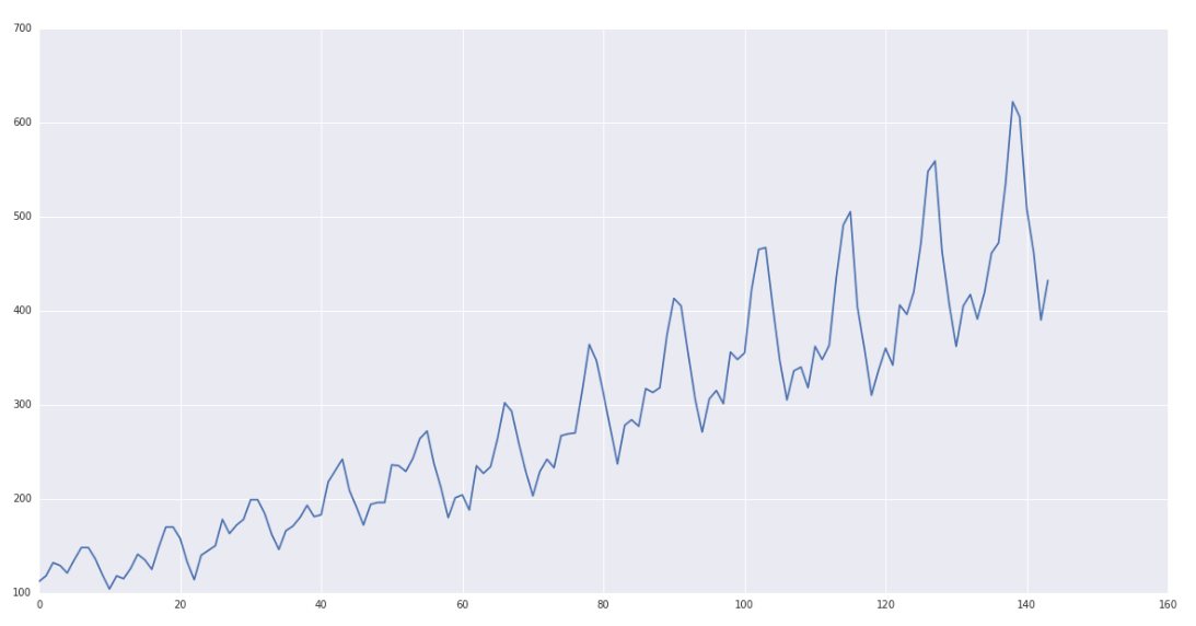
From intuition, we can see that there is pattern over here: (1) there exists an upward trend; (2) there exists seasonal fluctuation every once a while. However, this time series is not stationary.

[3] gives an excellent explanation for the meaning of a stationary time series:

Screenshot from 2017-07-26 20:46:35

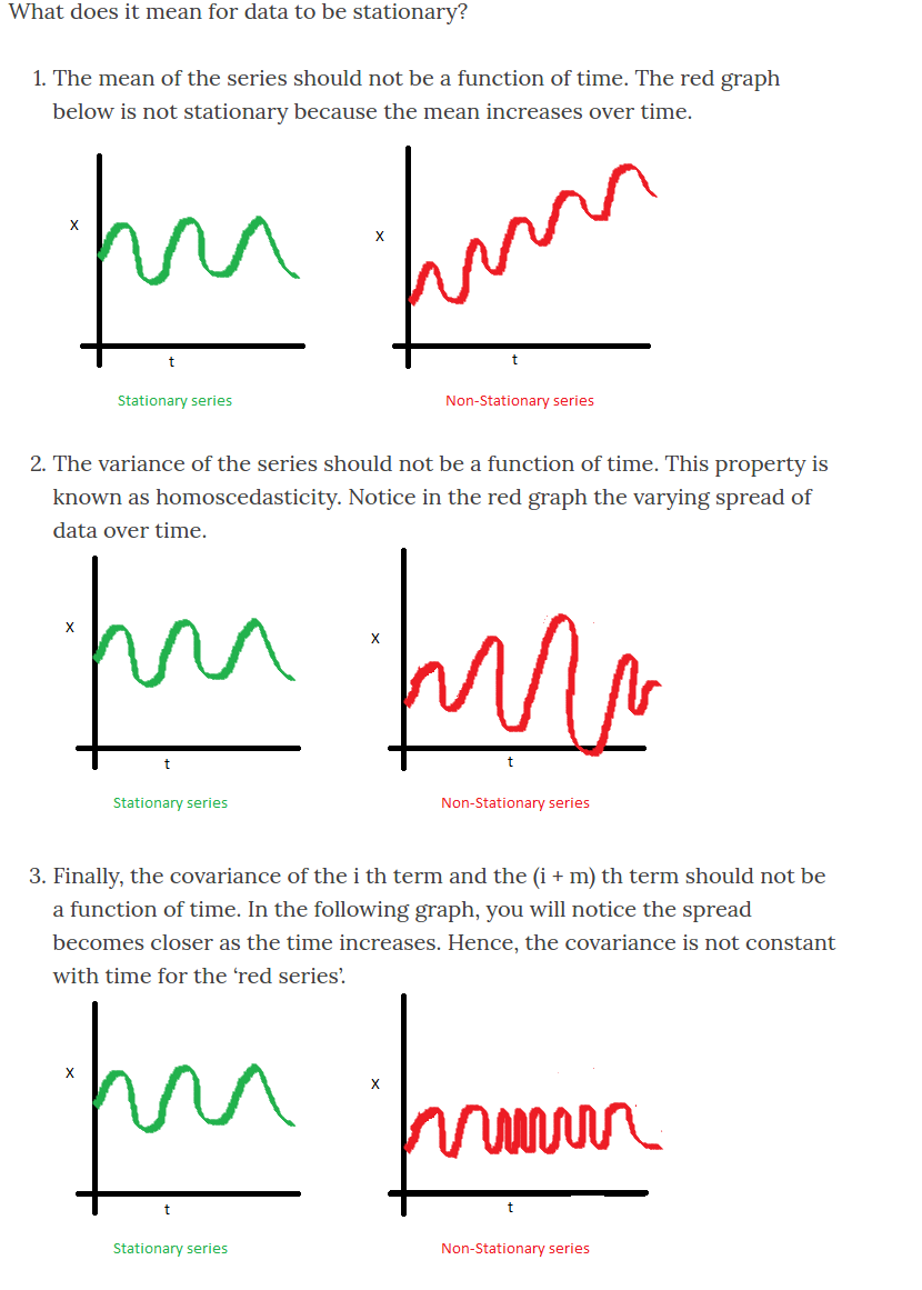
To put it mathematically, a stationary time series is:

$latex E(Y_1) = E(Y_2) = E(Y_3) = \cdots = E(Y_t) = \text{constant}$
$latex Var(Y_1) = Var(Y_2) = Var(Y_3) = \cdots = Var(Y_t)= \text{constant}$
$latex Cov(Y_1, Y_{1+k}) = Cov(Y_2, Y_{2+k}) = Cov(Y_3, Y_{3+k}) = \cdots = \gamma_k$ (depending only on lag $latex k$)

And also compare a stationary time series with white noise:

Let $latex \{\epsilon_t\}$ denote such a series then it has zero mean $latex E(\epsilon_t)=0$, $latex Var(\epsilon_t)=0$ for $latex \forall t$ and $latex E(\epsilon_t \epsilon_s)=0$ for $latex \forall t,s$.

The typical steps to perform time series analysis are as follows:

check whether it is a white noise time series. If it is, just stop, because there is no way that you can predict noise. (In practice, however, it is hard to determine whether a time series is white noise just by observing with eyes. So, my suggestion is to go ahead assuming this is a valid time series, and use cross validation to check if there exists any model that can successfully predict the time series.)
if this is a valid but non-stationary time series, make it stationary
build predictive models on the stationary time series

Here is my understanding why we need to make a time series stationary before training a model. Suppose your time series varies a lot much in a specific time range. If we build a linear regression model based on the mean square error loss, the errors from that time range will dominate the mean square error and force the weight adjustment more biased to the time range. However, we want to build a predictive model that can predict the time series equally well at any time point.

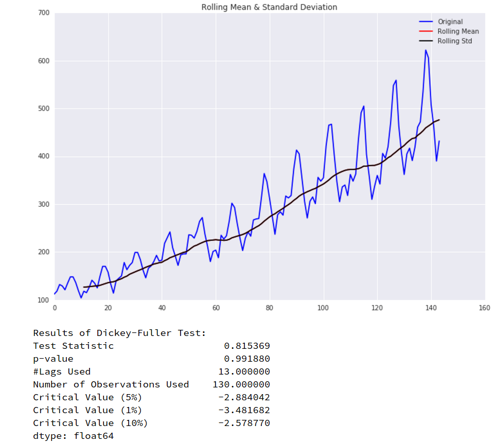
We can easily detect whether a time series is stationary using a helper function `test_stationarity` from [3] and [4]. The usage of `test_stationarity` is that if the ‘Test Statistic’ is greater than the ‘Critical Value’, or ‘p-value’ is well below a convincing threshold (say 0.05), then the time series is stationary.

Base on the raw time series, we use test_stationarity and find it is not stationary:

Screenshot from 2017-07-26 21:43:24

The techniques that you can use to make a time series stationary: (1) logarithmic; (2) first difference; (3) seasonal difference. See [4] and [5] for more techniques to make time series stationary.

ARIMA

Autoregressive integrated moving average (ARIMA) model assumes each time step $latex Y_t$ is a linear function of previous time steps $latex Y_{t-1}, Y_{t-2},\cdots$ and error terms $latex \epsilon_{t}, \epsilon_{t-1}, \epsilon_{t-2}, \cdots$. An ARIMA model(p, q, d) first applies $latex d$-difference on itself to obtain $latex \{Y_{t}\}$ and then assume:

$latex Y_t =\beta_0 + \beta_1 Y_{t-1} + \beta_2 Y_{t-2} + \cdots + \beta_p Y_{t-p} + \epsilon_t+ \Phi_{1} \epsilon_{t-1} + \Phi_{2} \epsilon_{t-2} + \cdots + \Phi_{q} \epsilon_{t-q} &s=2$

Here, the error term $latex \{\epsilon_t\}$ is not the error term from the Autoregressive (AR) model. Instead $latex \{\epsilon_t\}$ are estimated purely from data [11].

To determine the lag parameter $latex p$ in AR model, we can use autocorrelation_plot from pandas.autocorrelation_plot, which is the same thing as Autocorrelation Function (ACF) from statsmodels:

Autocorrelation plots are often used for checking randomness in time series. This is done by computing autocorrelations for data values at varying time lags. If time series is random, such autocorrelations should be near zero for any and all time-lag separations. If time series is non-random then one or more of the autocorrelations will be significantly non-zero. Therefore, autocorrelation can be used as a tool to quickly check whether your time series is suitable to use machine learning models to forecast. After all, if your time series is just white noises, it is meaningless to do time series forecast. The horizontal lines displayed in the plot correspond to 95% and 99% confidence bands. The dashed line is 99% confidence band.

Note that the ACF from statsmodels provides a parameter unbiased. If True, the plot will automatically adjust for the length of the time series. [14]

To determine the lag parameter $latex q$ in MA model, we can use Partial Autocorrelation Function (PACF) in statsmodels.

The rules to derive right $latex p$ and $latex q$ can be found from [12].

Screenshot from 2017-07-27 12:53:54

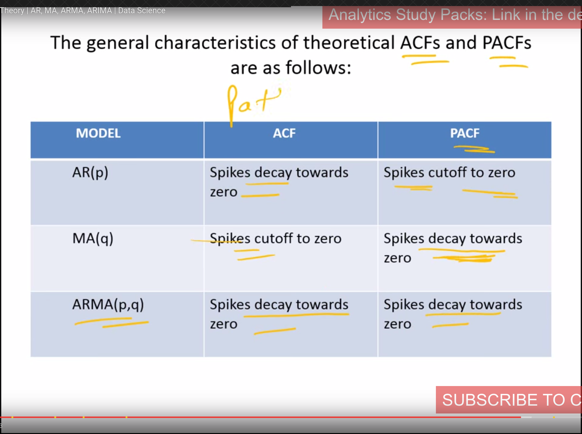
On the other hand, [4] points out that $latex p$ should be the value when the PACF chart crosses the upper confidence interval for the first time. $latex q$ should be the value when the ACF chart crosses the upper confidence interval for the first time. (Also see [15])

In my opinion, deriving $latex p$ and $latex q$ from observing ACF and PACF plots is a very ad-hoc, vague method. I’d prefer to do grid search on parameters as in [13] then filter out the best model according to AIC or similar metrics.

From [13]: AIC (Akaike Information Criterion) value, which is conveniently returned with ARIMA models fitted using statsmodels. The AIC measures how well a model fits the data while taking into account the overall complexity of the model. A model that fits the data very well while using lots of features will be assigned a larger AIC score than a model that uses fewer features to achieve the same goodness-of-fit.

Seasonality plot allows you to separate trend, seasonality and residual from a time series. According to [10], a time series consists of four components:

level, the average value in the series
trend, the increasing or decreasing value in the series
seasonality, the repeating short-term cycle in the series
noise, the random variation in the series

Below is the seasonality plot based on our data:

Screenshot from 2017-07-27 14:29:19

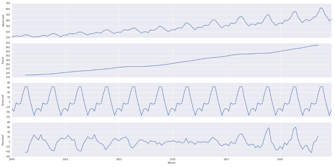
The residual is thus the combination of level and noise. One thing that I am not sure is how to use seasonality plot. One possible way is to fit ARIMA on residual because that’s the thing de-trended and de-seasonalized (see one person asked in a comment [8]). However, since the residual is already the level (seen as a constant?) + noise, is there any point to fit ARIMA? Also, even if we can fit an ARIMA on the residual, when we use it to predict the future, how can we transform the predicted value back to the raw scale? [15] actually supports this direction and also mentions the same concern: “Now that you have stationarized your time series, you could go on and model residuals (fit lines between values in the plot). However, as the patterns for the trend and seasonality information extracted from the series that are plotted after decomposition are still not consistent and cannot be scaled back to the original values, you cannot use this approach to create reliable forecasts“. Another direction is to use exogenous variables to fit the residuals, treating them as something not predictable by the time series itself [3]. However, we also face the same issue about how to transfer the predicted residuals back to the raw scale.

There are also other resources introducing seasonality decomposition, such as [9].

Based on what I’ve read so far, I’d say using seasonality plot as an exploration tool. But do not rely on it to train forecast model. After all, modern python ARIMA APIs integrates fitting trend and seasonality at the same time so that you don’t need to separate them out manually [7].

Reference:

[1] http://machinelearningmastery.com/time-series-prediction-with-deep-learning-in-python-with-keras/

[2] http://pandasplotting.blogspot.com/2012/06/autocorrelation-plot.html

[3] http://www.seanabu.com/2016/03/22/time-series-seasonal-ARIMA-model-in-python/

[4] https://www.analyticsvidhya.com/blog/2016/02/time-series-forecasting-codes-python/

[5] http://people.duke.edu/~rnau/whatuse.htm

[6] http://www.statsmodels.org/dev/generated/statsmodels.tsa.arima_model.ARIMA.html

[7] http://www.statsmodels.org/dev/generated/statsmodels.tsa.statespace.sarimax.SARIMAX.html

[8] https://stats.stackexchange.com/questions/223117/forecasting-residuals-from-seasonal-decomposition-appears-to-be-highly-auto-cor

[9] http://www.cbcity.de/timeseries-decomposition-in-python-with-statsmodels-and-pandas

[10] http://machinelearningmastery.com/decompose-time-series-data-trend-seasonality/

[11] https://stats.stackexchange.com/questions/26024/moving-average-model-error-terms/74826#74826