In the last weekend, I’ve struggled with many concepts in Reinforcement Learning (RL) and Dynamic Programming (DP). In this post, I am collecting some of my thoughts about DP, RL, Prioritized Sweeping and Prioritized Experience Replay. Please also refer to a previous post written when I first learned RL.
Let’s first introduce a Markov Decision Process $latex \mathcal{M} = (\mathcal{S}, \mathcal{A}, T, R)$, in which $latex \mathcal{S}$ is a set of states, $latex \mathcal{A}$ is set of actions, $latex T(s, a, s’)$ is transition function and $latex R(s,a,s’)$ is reward function. The value function of a state under a specific policy $latex \pi$, $latex V^\pi(s)$, is defined as the accumulated rewards from now on: $latex V^\pi(s)=\mathbb{E}(\sum\limits_{i=0}\gamma^i r_i | s_0 = s, \pi) &s=2$, where $latex 0 < \gamma < 1$ is a reward discount factor. $latex V^\pi(s)$ satisfies the Bellman equation: $latex V^\pi(s)=\mathbb{E}_{s’ \sim T(s,a,\cdot)}\{R(s,a,s’)+\gamma V^\pi(s’)\} &s=2$, where $latex a=\pi(s)$. The optimal value function is defined as $latex V^*(s) = max_\pi V^\pi(s)$. $latex V^*(s)$ also satisfies the Bellman equation: $latex V^*(s) = max_a \mathbb{E}_{s’ \sim T(s,a,\cdot)}\{R(s,a,s’) + \gamma V^*(s’)\} &s=2$. Another type of function is called Q-function, which is defined as the accumulated rewards for state-action pairs (rather than states themselves). The formulas of $latex Q^\pi(s,a)$ and $latex Q^*(s,a)$ are omitted here but can be found in many RL materials, such as [2].
DP refers to a collection of algorithms to find the optimal policy $latex \pi^*: \pi^*(s) = argmax_a \sum_{s’}T(s,a,s’) [R(s,a,s’) + \gamma V^*(s’)] &s=2$ for $latex \forall s \in \mathcal{S} &s=2$ when the transition function $latex T(s,a,s’)$ and reward function $latex R(s,a,s’)$ are known. Therefore, DP algorithms are also called model-based algorithms. (you assume you know or you have a model to predict $latex T(s,a,s’)$ and $latex R(s,a,s’)$ . And during policy search, you use the two functions explicitly.)
The simplest idea of DP is policy iteration as a synchronous DP method.
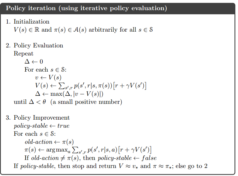
Here, we evaluate the value function under the current policy first (policy evaluation). Then, we update the current policy based on the estimated value function (policy improvement). The two processes alternate until the policy becomes stable. In synchronous DP method, states are treated equally and swept one by one.
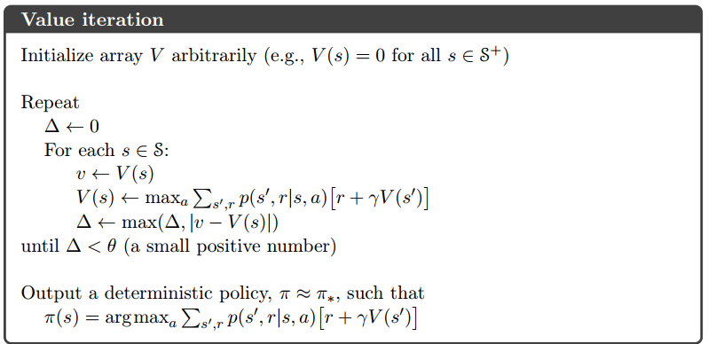
The drawback of policy iteration DP is that you need to evaluate value functions for all states for each intermediate policy. This possesses a large computational requirement if the state space is large. Later, people find a more efficient way called value iteration DP, in which only one sweep over the whole space of states is needed until the optimal policy is found:
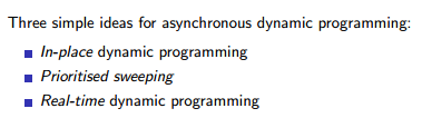
Even in value iteration, you still need to sweep over the whole space of states. To further accelerate that, people propose asynchronous DP: “These algorithms back up the values of states in any order whatsoever, using whatever values of other states happen to be available. The values of some states may be backed up several times before the values of others are backed up once. … Some states may not need their values backed up as often as others. We might even try to skip backing up some states entirely if they are not relevant to optimal behavior. ” (from [1])
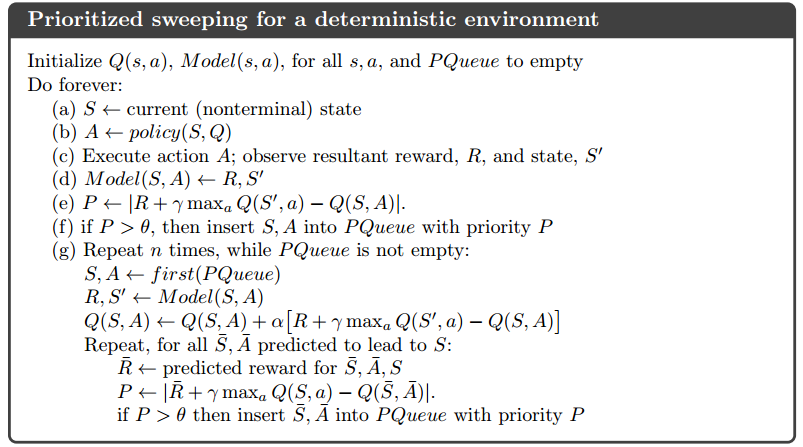
Prioritized sweeping is one asynchronous DP method [3]:
The goal of prioritized sweeping is to learn $latex V^*(s)$. The basic idea of it is to make some updates more urgent than others. The urgent updates are with large Bellman error, $latex err(s)=|V^*(s) – max_a Q^*(s,a)|$. The pseudo-code of it as in the original paper [4]:
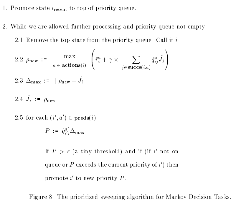
Something I am not sure is what policy is used during the learning. I think the policy is always the greedy policy $latex \pi^*: \pi^*(s) = argmax_a \sum_{s’}T(s,a,s’) [R(s,a,s’) + \gamma V^*(s’)] &s=2$ with some exploration stimulus (see the original paper [4] for the parameter $latex r_{opt}$ and $latex T_{bored}$).
[1] gave a slightly different prioritized sweeping when we focus on the Bellman error of Q function, rather than V function (note that this version of prioritized sweeping is still a DP, model-based algorithm because you need a transition function to know $latex \bar{S}$, $latex \bar{A}$ which lead to $latex S$ and a reward function to predict reward $latex \bar{R}$ for $latex \bar{S}, \bar{A}, S$):
Now, all above are DP methods, assuming you know $latex T(s,a,s’)$ and $latex R(s,a,s’)$ or you have a model to approximate the two functions.
RL methods are often called model-free methods because they don’t require you to know $latex T(s,a,s’)$ and $latex R(s,a,s’)$. $latex TD(0)$ or $latex TD(\lambda)$ are a type of algorithms to evaluate value function for a specific policy in an online fashion:
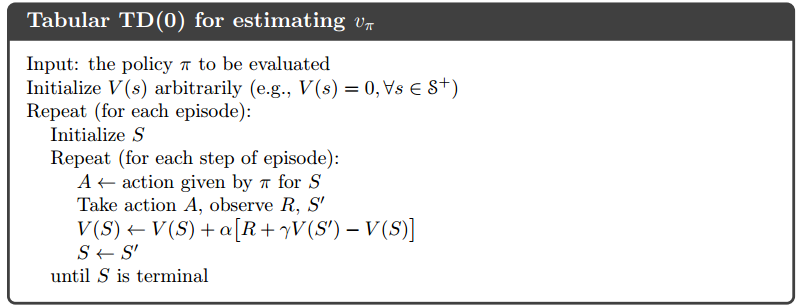
Note that, in the iterative update formula $latex V(S) \leftarrow V(S)+\alpha [R + \gamma V(S’) – V(S)]$ there is no longer reward function or transition function present as in DP-based methods.
$latex TD(0)$ (or more general $latex TD(\lambda)$) only solves the prediction problem, i.e., estimation value function for a specific policy $latex \pi$. Therefore, in theory you can’t use it to derive a better policy, i.e., solving a control problem. However, people still use it to find a good policy if a near-optimal policy is used when evaluating value functions and in addition you know reward/transition functions. This is a common scenario for games with predictable outcomes for each move, such as board games. During the learning, people can apply a near-optimal policy (e.g., $latex \epsilon$-greedy) to evaluate values of game states. In real games after the learning, the player evaluates the resulting state after each available movement and goes with the movement with the highest sum of immediate reward and resulting state value: $latex \pi(s) = argmax_a \sum_{s’}T(s,a,s’) [R(s,a,s’) + \gamma V(s’)] &s=2$. Of course, you are using the value function under the near-optimal policy to guide you select actions in the greedy policy. The value functions under two different policies might not totally agree with each other but in practice, you often end up with a good outcome. (I am not 100% confident about this paragraph but please also refer to [5] and a student report [9])
The policy iteration and value iteration in model-free RL algorithms correspond to SARSA and Q-learning [2]. I am omitting the details of them. Prioritized Experience Replay [8] bears the similar idea as in Prioritized Sweeping but applies on model-free contexts.
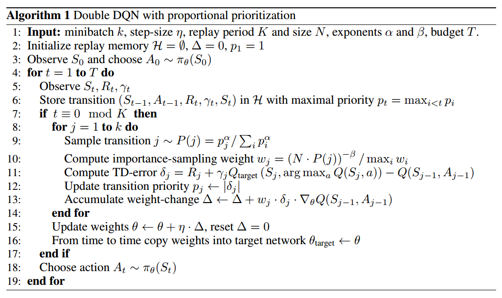
You can see that neither reward function nor transition function is needed in Prioritized Experience Replay.
Reference
[1] Richard S. Sutton’s book: Reinforcement Learning: An Introduction
[2] Reinforcement learning and dynamic programming using function approximators
[3] http://www.teach.cs.toronto.edu/~csc2542h/fall/material/csc2542f16_MDP2.pdf
[4] Prioritized Sweeping: Reinforcement Learning with Less Data and Less Real Time
[5] Self-Play and Using an Expert to Learn to Play backgammon with temporal difference learning
[7] https://stackoverflow.com/questions/45231492/how-to-choose-action-in-td0-learning
[8] Prioritized Experience Replay
[9] Reinforcement Learning in Tic-Tac-Toe Game and Its Similar Variations