Monte Carlo Tree Search Overview

Monte Carlo Tree Search (MCTS) has been successfully applied in complex games such as Go [1]. In this post, I am going to introduce some basic concepts of MCTS and its application.

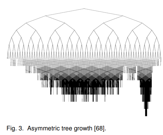
MCTS is a method for finding optimal decisions in a given domain by taking random samples in the decision space and building a search tree according to the results. Search trees are built to gradually cover the search space and in an iterative fashion:

Screenshot from 2018-04-13 18-19-18

and may result into asymmetric structure:

Screenshot from 2018-04-14 22-34-25

Each iteration is grouped by four phases, selection, expansion, simulation and backpropagation [4]:

Screenshot from 2018-04-14 22-39-08

Screenshot from 2018-04-14 22-39-16

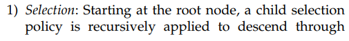
The tree policy and default policy may be defined differently in variations of MCTS. However they all rest on two fundamental concepts: the true value of an action may be approximated using random simulation; and that these values may be used efficiently to adjust the policy towards a best-first strategy [4].

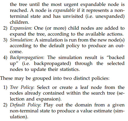
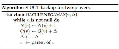
One most widely used variation of MCTS is UCT (Upper Confidence Bounds for Trees), whose tree policy is to select leaf nodes according to a multi-armed bandit metric called UCB1. The pseudo-code is given by [4]:

Screenshot from 2018-04-14 22-00-02

MCTS’s recent application in Go actually come from three papers [1] (AlphaGo), [2] (AlphaGo Zero), and [9] (AlphaZero). Let’s look at the first paper first [1], in which there are several networks trained:

1) a supervised learning policy network $p_{\sigma}$ . This is a straightforward, as its input is the board state $s$ (plus some move history and human engineered features) and its output is the action $a$ to take. The training data is essentially state-action pairs $(s, a)$ sampled from real human play matches. The goal of this supervised learning policy network is to accurately predict moves. Therefore, it is designed with convoluted structures with 13 layers. As reported, it can achieve 55.7% accuracy and takes 3ms per prediction.

2) a fast supervised learning policy network $p_{\pi}$ , which results in simpler structure, faster prediction time but less accuracy. It requires 2us per prediction and has 24.2% accuracy reportedly.

3) a policy network $p_{\rho}$ trained based on the supervised learning policy network $p_{\sigma}$ and by Reinforcement Learning (more specifically, policy gradient method [3]). I think this is a smart choice: if you train a policy network by RL from scratch you may not end up learning well because the game is too complex such that the network will take long time until it adjusts its weights to some meaningful values. Initializing the weights of $p_{\rho}$ to $p_{\sigma}$ is like an effective bootstrapping. On the other hand, $p_{\sigma}$ ‘s goal is simply achieving prediction accuracy as high as possible, rather than our real goal for winning. The RL-based policy network would adjust the network to fully align with the goal of winning. Thus, a trained $p_{\rho}$ should perform stronger than $p_{\sigma}$ .

4) a value network $v_\theta(s)$ which estimates the expected outcome from position $s$ played by using the RL policy network $p_{\rho}$ for both players: $v^{p_{\rho}}(s) = \mathbb{E}[z_t | s_t=s, a_{t \cdots T} \sim p_{\rho}]$ . As the paper [1] stated, the most useful value network should estimate the expected outcome under perfect play, $v^*(s)$ , which means each of the two players acts optimally to maximize his own winning probability. But since we do not have perfect play as ground truth, we have to use $p_{\rho}$ to generate gameplay data. Therefore, we have $v_\theta(s) \approx v^{p_{\rho}}(s) \approx v^*(s)$ . But note that, training a value network is not the only way to estimate $v^{p_{\rho}}(s)$ . We can also use Monte Carlo rollouts to simulate a large number games by using $p_{\rho}$ . However it takes much larger computational resource.

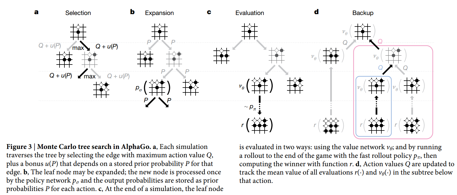
After training the four networks, MCTS will base on these networks to select actions by lookahead search. Let’s look at a typical iteration of MCTS in Alphago:

Screenshot from 2018-04-13 18-22-26

You could think in such way that each node in the search tree maintains two values $N(s,a)$ and $Q(s,a)$ :

Screenshot from 2018-04-13 18-24-26

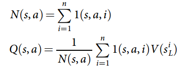
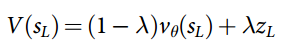
where $V(s_L^i)$ is the value of the leaf state after the selection phase in simulation $i$ . $V(s_L^i)$ combines the estimated outcome from $v_\theta$ and a roll out outcome $z$ using the fast policy network $p_\pi$ :

Screenshot from 2018-04-13 18-24-32

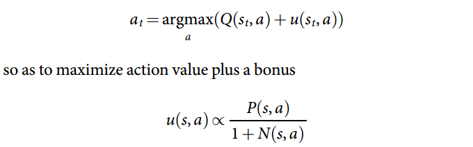
Maintaining $Q(s,a)$ and $N(s,a)$ is primarily for defining the tree policy, the policy used to navigate nodes in the selection phase. Specifically, at each time step $t$ during the selection phase of a simulation, an action $a_t$ is selected according to:

Screenshot from 2018-04-13 18-44-53

This is a little different than UCB1 (Upper Confidence Bound) used in UCT (Upper Confidence Bounds for Trees), a common version of MCTS that characterizes using UCB1 in the selection phase [4]:

Screenshot from 2018-04-13 18-59-25

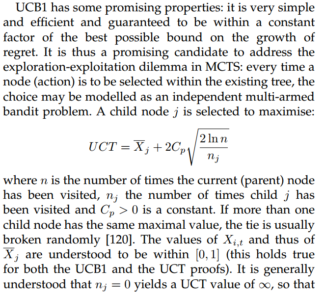
However, both AlphaGo’s MCTS and UCT share the same idea as to model the action choice in the selection phase as a bandit problem. As such, the action values dynamically change according to historically received average rewards, as well as the number of total trials and trials for that action specifically.

In summary, AlphaGo’s MCTS actually only uses two networks ( $p_\pi$ and $v_\theta$ ) from the four trained networks ( $p_\sigma$ , $p_\pi$ , $p_\rho$ , and $v_\theta$ ). The two networks $p_\pi$ and $v_\theta$ are only used in the leaf evaluation function $V(s^L)$ .

AlphaGo also embodies two principles of reducing the search space in MCTS. First, to reduce the breadth of search, it selectively pick and expand the action nodes based on the action values calculated as a bandit problem. Additionally, in the simulation (evaluation) phase, the rollout uses the fast policy network $p_\pi$ to sample actions which also reduces the breadth of the search. Second, to reduce the depth of search, it relies on the leaf evaluation function $V(s^L)$ to evaluate the board value (combined with just one roll out, instead of fully relying on a large number of rollouts).

Now, let’s look at the second version AlphaGo, which is called AlphaGo Zero [2]. The most significant change is that AlphaGo Zero does not require any human play data as in AlphaGo to bootstrap itself. AlphaGo Zero gets rid of training multiple networks but only keeps one unified neural network $f_\theta$ which learns to output two heads: (1) an action probability distribution ( $\vec{p}$ , a vector, whose component is $p_a = Pr(a|s)$ ); (2) and outcome value prediction ( $v$ , a scalar).

The neural network $f_\theta$ gets initialized with random weights and will be updated in iterations. Self-play data are generated by two Go AI bots which equip the same neural network snapshot. The neural network snapshot is picked periodically as the best performant player seen so far in all previous iterations. Let us denote the picked snapshot as $\alpha_{\theta_{i-1}} = argmax_i \; performance(f_{\theta_i})$ . At each move, an MCTS search is executed based on $\alpha_{\theta_{i-1}}$ in the simulation phase. The output of the MCTS search is an action distribution $\vec{\pi}$ determined by the upper confidence bound for each action: $Q(s,a)+U(s,a)$ where $U(s,a) \propto P(s,a)/(1+N(s,a))$ , the same bound metric as in AlphaGo [1].

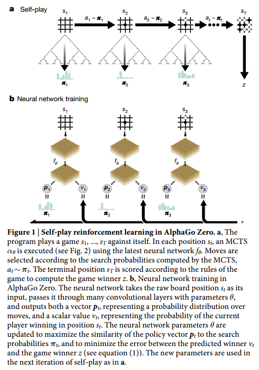
When such self-play proceeds to the game end, we store the game outcome $z$ and each of the previous MCTS action distributions as a distribution-outcome tuple $(\vec{\pi}_t, z)$ . These distribution-outcome tuples will serve as the training data for updating the weights of $f_\theta$ . The full procedure is illustrated below:

Screenshot from 2018-04-14 10-06-22

The third version, AlphaZero [9], has further differences than AlphaGo Zero:

AlphaZero is more general, which can be applied to other different games such as chess and shogi. It achieves so by supporting evaluating non-binary game outcomes and less exploiting game-specific training tricks.
In AlphaGo Zero, self-play games were generated by the selected snap of the best player from previous iterations. In contrast, AlphaZero simply maintains a single neural network that is updated continually. So self-play games are always generated by the latest parameters for this neural network.

MCTS convergence

According to [5,6], in UCT, the failure probability at the root of the tree (i.e., the probability of selecting a suboptimal action) converges to zero at a polynomial rate as the number of games simulated grows to infinity. In a two-person zero-sum game, this means UCT converges to the minimax algorithm’s solution, which is the optimal move if both players are under perfect play, which is also the move to minimize the maximal possible loss the opponent can exert.

Here, I am using a small example to sketch why UCT could converge to minimax. First, the following plot shows a minimax tree for a game. Each of two players makes exactly one move until the game ends. The numbers in the circles indicate the reward to the player. Solid lines indicate the actual moves selected under perfect play by both players.

minimax

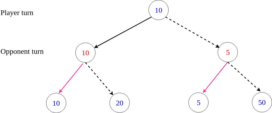
Now, suppose we start to build a UCT. Since UCT has the exploration term $2 C_p \sqrt{\frac{2 \ln n}{n_j}}$ , we could imagine that at some point each terminal state has been visited once:

mcts (1)

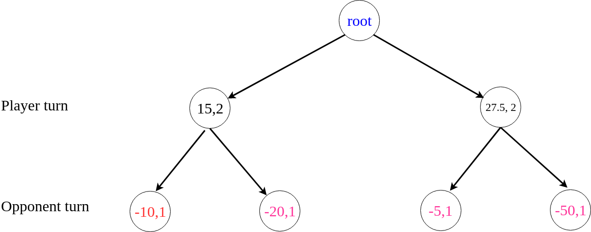
Here in each circle there is a tuple indicating the average reward and visited times on that node. If MCTS stops at this moment, it seems like the player would choose the right action because it has a higher average reward, which is different than the minimax solution.

However, after that, UCT would traverse the node (-5,1) much more frequently than the node (-50,1). Therefore, The node (27.5, 2) will eventually converge to its real reward 5.

Reference

[1] Silver, D., Huang, A., Maddison, C. J., Guez, A., Sifre, L., Van Den Driessche, G., … & Dieleman, S. (2016). Mastering the game of Go with deep neural networks and tree search. nature, 529(7587), 484-489.

[2] Silver, D., Schrittwieser, J., Simonyan, K., Antonoglou, I., Huang, A., Guez, A., … & Chen, Y. (2017). Mastering the game of go without human knowledge. Nature, 550(7676), 354.

[3] https://czxttkl.com/?p=2812

[4] Browne, C. B., Powley, E., Whitehouse, D., Lucas, S. M., Cowling, P. I., Rohlfshagen, P., … & Colton, S. (2012). A survey of monte carlo tree search methods. IEEE Transactions on Computational Intelligence and AI in games, 4(1), 1-43.

[5] Kocsis, L., Szepesvári, C., & Willemson, J. (2006). Improved monte-carlo search. Univ. Tartu, Estonia, Tech. Rep, 1.

[6] Kocsis, L., & Szepesvári, C. (2006, September). Bandit based monte-carlo planning. In European conference on machine learning (pp. 282-293). Springer, Berlin, Heidelberg.

[9] Silver, D., Hubert, T., Schrittwieser, J., Antonoglou, I., Lai, M., Guez, A., … & Hassabis, D. (2017). Mastering chess and shogi by self-play with a general reinforcement learning algorithm.