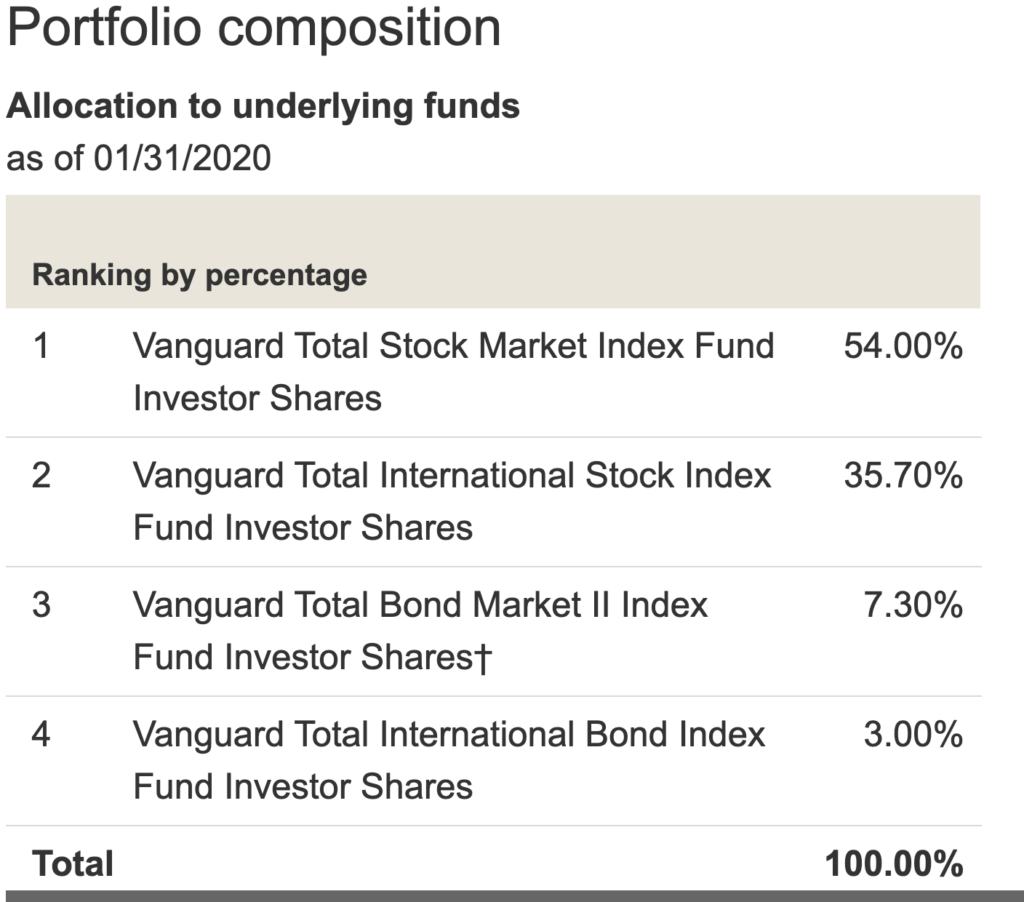
There are several online posts [1][2] that illustrate the idea of Transformer, the model introduced in the paper “attention is all you need” [4].
Based on [1] and [2], I am sharing a short tutorial for implementing Transformer [3]. In this tutorial, the task is “copy-paste”, i.e., to let a Transformer learn to output the same sequence as the input sequence. We denote the symbols used in the code as:
| Name | Meaning |
| src_vocab_size=12 | The vocabulary size of the input sequence |
| tgt_vocab_size=12 | The vocabulary size of the output sequence. Since our task is to copy the input sequence, tgt_vocab_size = src_vocab_size. We reserve symbol 0 for padding and symbol 1 for the decoder starter symbol, and we assume possible real symbols are from 2 to 11. Therefore, the total vocabulary size is 12. |
| dim_model=512 | This is the dimension of the embedding, as well as the output of self-attention, and the input/output of the position-wise feed forward model. |
| dim_feedforward=256 | The size of the hidden layer in the position-wise feed forward layer. |
| d_k = 64 | The dimension of each attention head. |
| num_heads=8 | The number of attention heads. For the sake of computational convenience, d_k * num_heads should be equal to dim_model. |
| seq_len=7 | The length of input sequences |
| batch_size=30 | Batch size, the number of input sequences per batch |
| num_stacked_layers=6 | The number of layers to be stacked in both Encoder and Decoder |
Let’s first look at what the input/output data looks like, which is generated by data_gen. Each Batch instance contains several essential pieces of information to be used in training:
- src (batch_size x seq_len): the input sequence to the encoder
- src_mask (batch_size x 1 x seq_len): the mask of the input sequence, so that each input symbol can fine control which other symbols to attend
- trg_y (batch_size x seq_len): the output sequence as the label, which is the same as src given that our task is simply “copy-paste”
- trg (batch_size x seq_len): the input sequence to the decoder. The first symbol of each sequence is symbol 1 that helps kicking off the decoder; the last symbol of each sequence is the second to the last of the trg_y sequence.
- trg_mask (batch_size x seq_len x seq_len): the mask of the output sequence, so that at each decoding step, a symbol being decoded can attend to other already decoded symbols.
trg_mask[i, j, k], a binary value, indicates whether in the i-th output sequence the j-th symbol can attend to the k-th symbol. Since a symbol can attend all its preceding symbols,trg_mask[i,j,k]=1for allk <= j.
Now, let’s look at EncoderLayer class. There are num_stacked_layers=6 encoder layers in one Encoder. The bottom layer takes the symbol embeddings as input, while each of the upper layers takes the previous layer’s output. Both the symbol embedding and each layer’s output has the same dimension `batch_size x seq_len x dim_model`, so in theory you can stack as many layers as needed because they all have compatible input/output. The symbol embedding converts input symbols into embeddings, plus positional encoding which helps the model learns positional information.
One EncoderLayer does the following things:
- It has three matrices stored in
MultiHeadedAttention.linears[:3], which we call query transformation matrix, key transformation matrix, and value transformation matrix. They transform the input from the last layer into three matrices which the self-attention module will use. Each of the output matrices, which we call query, key, and value, has the shapebatch_size x num_heads x seq_len x d_k. - The transformed matrices are used as query, key, and value in self-attention (
attentionfunction). The attention is calculated based on Eqn.1 in [4]:

The attention function also needs a mask as input. The mask tells it for each symbol what other symbols it can attend to (due to padding, or other reasons). In our case, our input sequences are of the equal length and we allow all symbols attend to other symbols; so the mask is always filled with ones.
- The attentions of
d_kheads are concatenated and passed through a linear projection layer, which results to the output with shape `batch_size x seq_len x dim_model` - The output is finally processed by a BatchNorm layer and a Residual layer.
So far, the encoder part can be illustrated in the following diagram [1] (suppose our input sequence has length 2, containing the symbol 2 and 3):

One DecoderLayer does the following thing:
- it first does self-attention on the target sequence (
batch.trg, not thetrg_ysequence), which generates attention of shape (batch_size, seq_len, dim_model). The first symbol of a target sequence is 1, a symbol indicating the decoder to start decoding. - the target sequence performs attention on the encoder, i.e., using the target sequence’s self attention as the query, and using the final encoder layer’s output as the key and value.
- Pass the encoder-decoder attention’s output through a feedforward layer, with batch norm and residual connection. The output of one DecoderLayer has the shape `batch_size x seq_len x dim_model`. Again this shape allows you stack as many layers as you want.
The decoder part is shown in the following diagram:

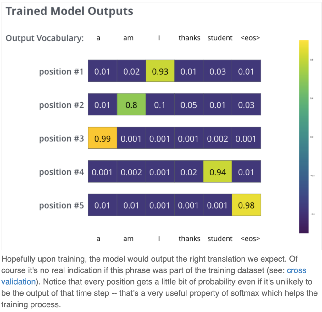
The last part is label fitting. The last layer of DecoderLayer has the output of shape , i.e., each target symbol’s attention. We pass them through a linear project then softmax such that each target symbol will be associated with a probability distribution of the next symbol to decode. We fit the probability distribution against batch.trg_y by minimizing the KL divergence. Here is one example of label fitting:
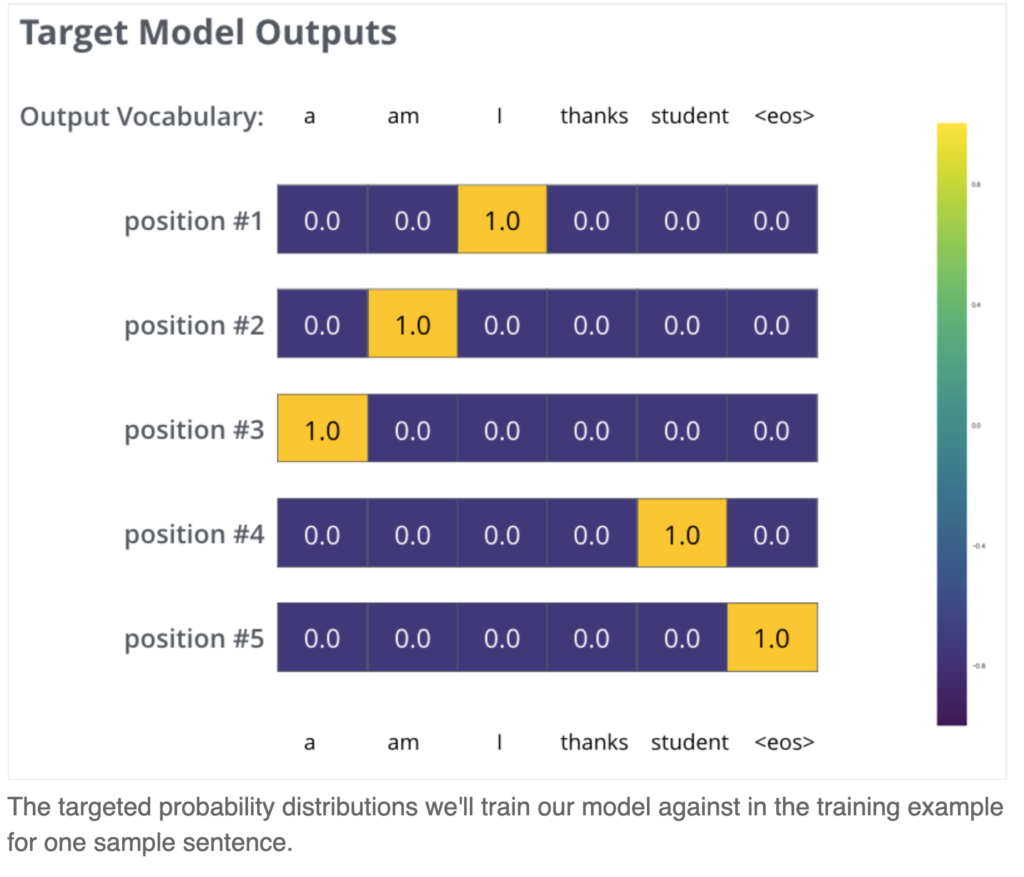
In practice, we also apply label smoothing such that the target distribution to fit has slight probability mass even on the non-target symbol. So for example, the target distribution of position #1 (refer to the diagram on the left) is no longer (0, 0, 1, 0, 0); rather it should be (0.1, 0.1, 0.6, 0.1, 0.1) if you use 0.1 label smoothing. The intuition is that even our label may not be 100% accurate and we should not let the model overly confident in the training data. In other words, label smoothing helps prevent overfitting and hope to improve generalization in unseen data.
[1] http://jalammar.github.io/illustrated-transformer/
[2] http://nlp.seas.harvard.edu/2018/04/03/attention.html
[3] https://github.com/czxttkl/Tutorials/blob/master/experiments/transformer/try_transformer.py


 represents
  ,
,  is the stationary distribution of Markov chain for
 ![V^\pi(s)=\mathbb{E}_{a \sim \pi}[G_t|S_t=s]](https://czxttkl.com/wp-content/ql-cache/quicklatex.com-81e80918e8ee5ee716538d3fd9167787_l3.png "Rendered by QuickLaTeX.com") , and
, and ![Q^{\pi}(s,a)=\mathbb{E}_{a \sim \pi}[G_t|S_t=s, A_t=a]](https://czxttkl.com/wp-content/ql-cache/quicklatex.com-fb78793408bc59dde51b8ee271d116f6_l3.png "Rendered by QuickLaTeX.com") .
.  is accumulated rewards since time step
  :
:  .
. is:
is:![\nabla_\theta J(\theta) = \mathbb{E}_{\pi}[Q^\pi(s,a)\nabla_\theta ln \pi_\theta(a|s)]](https://czxttkl.com/wp-content/ql-cache/quicklatex.com-be1e10121a356cdfda96fad1cd9046e7_l3.png "Rendered by QuickLaTeX.com")
 .
. means the state and action distribution is generated by following
  , then the objective function becomes:
![\nabla_\theta J(\theta) = \mathbb{E}_{s\sim d^\beta}[\sum\limits_{a\in A}\nabla_\theta \pi(a|s) Q^\pi(s,a) + \pi(a|s)\nabla_\theta Q^\pi(s,a)] \newline \approx \mathbb{E}_{s\sim d^\beta}[\sum\limits_{a\in A}\nabla_\theta \pi(a|s) Q^\pi(s,a)] \newline =\mathbb{E}_{\beta}[\frac{\pi_\theta(a|s)}{\beta(a|s)}Q^\pi(s,a)\nabla_\theta ln \pi_\theta(a|s)]](https://czxttkl.com/wp-content/ql-cache/quicklatex.com-45583aee57264f3e0f6b1e30d1398e67_l3.png "Rendered by QuickLaTeX.com")

 could incur some learning difficulty problems [5]:
 , thus

![\nabla_\theta J(\theta) = \int\limits_S d^\beta(s) \nabla_\theta Q^\mu(s, \mu_\theta(s)) ds \approx \mathbb{E}_\beta [\nabla_\theta \mu_\theta(s) \nabla_a Q^\mu(s,a)|_{a=\mu_\theta(s)}]](https://czxttkl.com/wp-content/ql-cache/quicklatex.com-95413f31d5976999e5fcb9526f93b1ca_l3.png "Rendered by QuickLaTeX.com")
 can be updated off policy. Because we only need to sample
  , then
  can be calculated without knowing what action the behavior policy
  ). We should also note that there is an approximation in the formula of
  , because
  cannot be applied chain rules easily since even you replace
  with
with  , the
, the  function itself still depends on
  on the optimal Q-function of policy governed by
 using
using  . Policy gradient methods do not depend on value functions to infer the best policy, instead they directly learn a probability function
  . However policy gradient methods may still learn value functions for the purpose of better guiding the learning of the policy probability function
  ,
,
![\nabla_\theta J(\theta) = \mathbb{E}_{s,a\sim\pi}[Q^\pi(s,a)\nabla_\theta log \pi_\theta(a|s)]](https://czxttkl.com/wp-content/ql-cache/quicklatex.com-2beb309a8f7f851c92dbb14d57dfb021_l3.png "Rendered by QuickLaTeX.com")
 : REINFORCE uses a Monte Carlo method in which empirical accumulated rewards
  and uses
  to approximate
  and uses
  to approximate
 ![\mathbb{E}_{s,a \sim \pi} [\cdot]](https://czxttkl.com/wp-content/ql-cache/quicklatex.com-5f964b41e5266ad100f51f229146af14_l3.png "Rendered by QuickLaTeX.com") , we need to collect on-policy samples. That’s why the soft actor-critic papers mentions in Introduction:
, we need to collect on-policy samples. That’s why the soft actor-critic papers mentions in Introduction: ,
, ![J(\theta)=\mathbb{E}_{s\sim \pi_b} \left[ \mathbb{E}_{a\sim\pi}Q^{\pi}(s,a) \right]](https://czxttkl.com/wp-content/ql-cache/quicklatex.com-87a3d46598262d6296e094b4f0577e4f_l3.png "Rendered by QuickLaTeX.com")
![\mathbb{E}_{a\sim\pi}[\cdot]](https://czxttkl.com/wp-content/ql-cache/quicklatex.com-ae63a6ea8b6c194261a8601712a0ab95_l3.png "Rendered by QuickLaTeX.com") because any such gradient can’t be computed using mini-batches collected from
because any such gradient can’t be computed using mini-batches collected from ![\mathbb{E}_{a\sim\pi}\left[ Q^{\pi}(s,a)\right]](https://czxttkl.com/wp-content/ql-cache/quicklatex.com-786220bca35e8ded97c42aa993eea6f2_l3.png "Rendered by QuickLaTeX.com") as
as ![\mathbb{E}_{a\sim\pi_b}\left[\frac{\pi(a|s)}{\pi_b(a|s)}Q^{\pi_b}(s,a) \right]](https://czxttkl.com/wp-content/ql-cache/quicklatex.com-3c2b92f89489c602968842cc5519c476_l3.png "Rendered by QuickLaTeX.com") . This results to the gradient update
. This results to the gradient update ![\mathbb{E}_{s,a \sim \pi_b} [\frac{\pi(a|s)}{\pi_b(a|s)} Q^{\pi_b}(s,a) \nabla_\theta log \pi(a|s)]](https://czxttkl.com/wp-content/ql-cache/quicklatex.com-e53e8508268cfd534fe9b14611870dd4_l3.png "Rendered by QuickLaTeX.com") . See [18]. However, importance sampling can cause great variance empirically.
. See [18]. However, importance sampling can cause great variance empirically.![J(\theta)=\mathbb{E}_{s\sim\pi_b}\left[Q^{\pi}(s,\pi(s))\right]](https://czxttkl.com/wp-content/ql-cache/quicklatex.com-1104f775b9ace7162e169ed09964c019_l3.png "Rendered by QuickLaTeX.com") . The gradient update can be computed as
. The gradient update can be computed as ![\mathbb{E}_{s\sim \pi_b}\left[ \nabla_\theta \pi(s) \nabla_a Q^\pi(s,a)|_{a=\pi(s)}\right]](https://czxttkl.com/wp-content/ql-cache/quicklatex.com-80844574a104283d7e501a74060dc13b_l3.png "Rendered by QuickLaTeX.com") . This is how DPG works. See [20].
. This is how DPG works. See [20]. , a deterministic function plus an independent noise, we would have
 ![J(\theta)=\mathbb{E}_{s\sim\pi_b, \epsilon \sim p_\epsilon}\left[Q^{\pi}(s,\pi(s))\right]](https://czxttkl.com/wp-content/ql-cache/quicklatex.com-786969025c9166246b593b6c0aab5fd0_l3.png "Rendered by QuickLaTeX.com") . The gradient update would be:
. The gradient update would be: ![\mathbb{E}_{s\sim\pi_b, \epsilon \sim p_\epsilon}\left[\nabla_a Q^{\pi}(s,a)|_{a=\pi(s)} \nabla_\theta \pi(s) \right] \newline=\mathbb{E}_{s\sim\pi_b, \epsilon \sim p_\epsilon}\left[\nabla_a Q^{\pi}(s,a)|_{a=\pi(s) } \nabla_\theta \pi^{deterministic}(s) \right]](https://czxttkl.com/wp-content/ql-cache/quicklatex.com-3e7b7d028abc02800aecea0e7c0aa695_l3.png "Rendered by QuickLaTeX.com")
![\[ J(\pi)=\sum\limits^T_{t=0}\mathbb{E}_{(s_t, a_t)\sim\rho_\pi} \left[r(s_t, a_t) + \alpha \mathcal{H} \left( \pi\left(\cdot | s_t \right) \right) \right], \]](https://czxttkl.com/wp-content/ql-cache/quicklatex.com-5423cd8c98adcc2ea0804f071ecc8266_l3.png "Rendered by QuickLaTeX.com")
 of an action distribution
  is the entropy defined as
 ![\mathbb{E}_{a \sim \pi(\cdot|s_t)}[-log \pi(a|s)]](https://czxttkl.com/wp-content/ql-cache/quicklatex.com-880d8a6d23e8e39d4ae342a2a93bd4db_l3.png "Rendered by QuickLaTeX.com") , and
, and  is the term controlling the influence of the entropy term.
 by subsuming it into the reward function. Therefore, with
 ![\[ J(\pi)=\sum\limits^T_{t=0}\mathbb{E}_{(s_t, a_t)\sim\rho_\pi} \left[r(s_t, a_t) + \mathcal{H} \left( \pi\left(\cdot | s_t \right) \right) \right] \]](https://czxttkl.com/wp-content/ql-cache/quicklatex.com-4a6cf3d3915c59fcec26e955409380eb_l3.png "Rendered by QuickLaTeX.com")
![\[ \mathcal{T}^\pi Q(s_t, a_t) \triangleq r(s_t, a_t) + \gamma \mathbb{E}_{s_{t+1}\sim p}\left[V(s_{t+1})\right] \]](https://czxttkl.com/wp-content/ql-cache/quicklatex.com-471e4ff56f93a3edf8422b21a37dd645_l3.png "Rendered by QuickLaTeX.com")
![\[ V(s_t) = \mathbb{E}_{a_t \sim \pi}\left[Q(s_t, a_t) - \log \pi(a_t|s_t) \right] \]](https://czxttkl.com/wp-content/ql-cache/quicklatex.com-a9bacc02a46af7eea5da40a110dae030_l3.png "Rendered by QuickLaTeX.com")
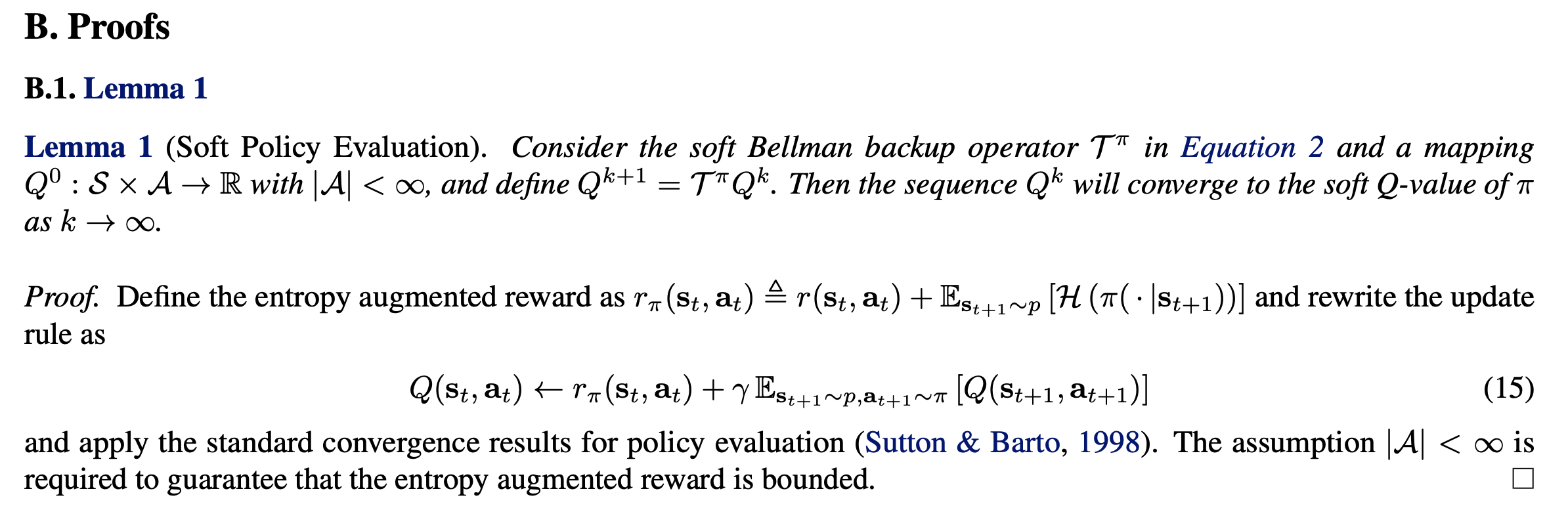
 because of the way we define Eqn.15: for each state
  equations in total. And there are
  , where
  is the operator for calculating expectation
 ![\mathbb{E}[\cdot]](https://czxttkl.com/wp-content/ql-cache/quicklatex.com-eff568ea1582b23954f9a75fe3009a12_l3.png "Rendered by QuickLaTeX.com") .
. is a
is a  -contraction under the infinity norm, i.e.,
  . Explained in plain English,
 from [7] and the fact that
  (because
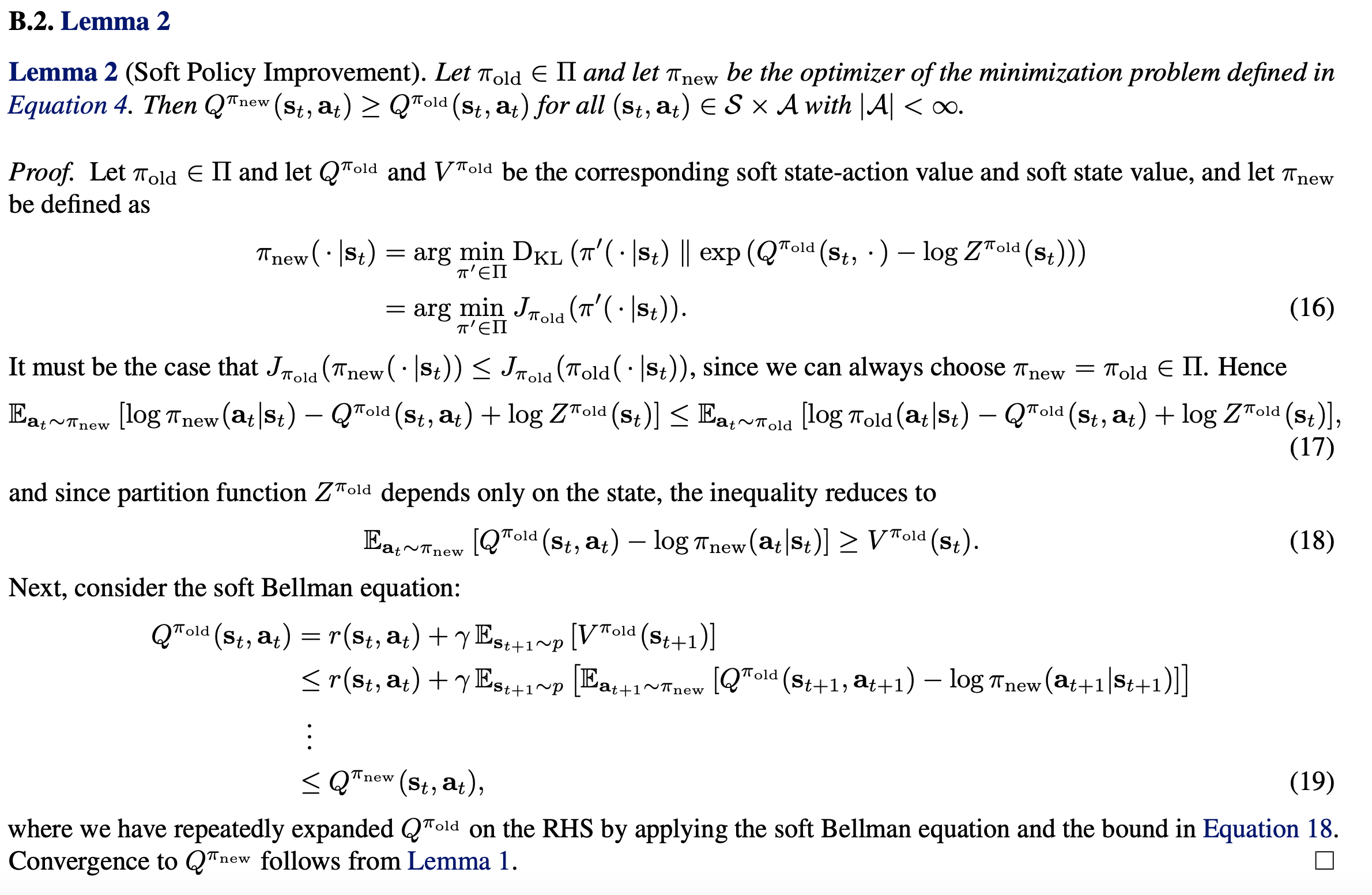
 -divergence formula
  . From Eqn. 16, we expand
 ![J_{\pi_{old}}(\pi'(\cdot|s_t)) \newline \triangleq D_{KL} (\pi'(\cdot | s_t) \; \Vert \; exp(Q^{\pi_{old}}(s_t, \cdot) - \log Z^{\pi_{old}}(s_t)) ) \newline = - \int \pi'(a_t | s_t) \log \frac{exp(Q^{\pi_{old}}(s_t, a_t) - \log Z^{\pi_{old}}(s_t)))}{\pi'(a_t|s_t)} d a_t \newline = \int \pi'(a_t | s_t) \big(\log \pi'(a_t|s_t) + \log Z^{\pi_{old}}(s_t) - Q^{\pi_{old}}(s_t, a_t) ) \big) d a_t \newline = \mathbb{E}_{a_t \sim \pi'}[\log \pi'(a_t|s_t) + \log Z^{\pi_{old}}(s_t) - Q^{\pi_{old}}(s_t, a_t) )]](https://czxttkl.com/wp-content/ql-cache/quicklatex.com-9326b886e89c908e7b8a582c210605dd_l3.png "Rendered by QuickLaTeX.com")
 , which is different than Eqn.1. The purpose of defining
  is to help us get to Eqn. 18, which is then used to prove
  in Eqn. 19.
 , and another output vector for action standard deviations
  . The action that is to be taken will be sampled from
  .
.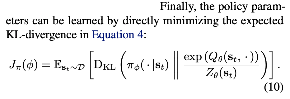
![D_{KL}(p\Vert q) = \mathbb{E}_{x \sim p(x)}[\log p(x) - \log q(x)]](https://czxttkl.com/wp-content/ql-cache/quicklatex.com-23d5ad1f4496452366a1d22e5299f373_l3.png "Rendered by QuickLaTeX.com") ,
,  can be rewritten as:
![J_\pi(\phi) = \mathbb{E}_{s_t \sim \mathcal{D}, a_t \sim \pi_\phi}[\log \pi_\phi(a_t | s_t) - Q_\theta(s_t, a_t)]](https://czxttkl.com/wp-content/ql-cache/quicklatex.com-ef7e892a4de4497d3a6a56ae0b2ade2e_l3.png "Rendered by QuickLaTeX.com")
 with a stochastic input
  . This trick is also widely used in variational autoencoders, and has been discussed in [11, 13, 14, 15, 16] . Reparameterization trick can also be illustrated in the diagram below [11]:
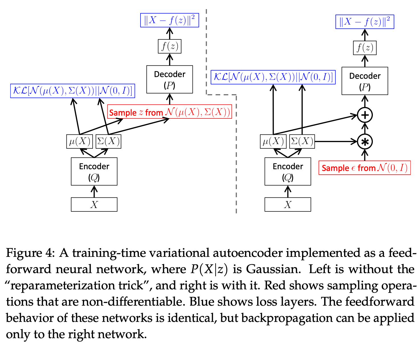
 :
:![\hat{\nabla}_\phi J_\pi(\phi) \newline = \nabla_\phi [\log \pi_\phi(a_t | s_t) - Q_\theta(s_t, a_t)] |_{a_t = f_\phi(\epsilon_t ; s_t)} \newline = (\nabla_{a_t} \log \pi_\phi(a_t | s_t) - \nabla_{a_t} Q_\theta (s_t, a_t)) \nabla_\phi f_\phi(\epsilon_t; s_t)](https://czxttkl.com/wp-content/ql-cache/quicklatex.com-ba5b4816d2d2c65a2dab0360ec29f073_l3.png "Rendered by QuickLaTeX.com")
 . Right now I am not sure why but I will keep figuring it out.
 also needs to account that. Basically, if squashed action = squash function(raw_action), then the probability density of squashed actions will be different than the probability density for raw actions [17]. The original code reflects this in

 . When
  , the formula becomes
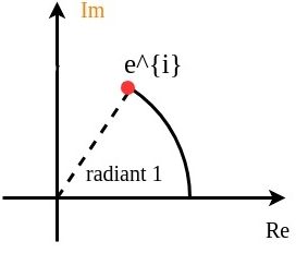
  known as Euler’s identity.
 when
when  ),
),
 with
with  , we have

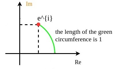
 as
as 
 and y coordinate
  on a unit circle (centered at the origin with radius 1) in the complex plane.
 describes the point that moves distance
  viewed in x&y coordinates:
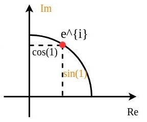
 means 1 is stretched to 8, or 1 is stretched to 2 first, then that point is stretched to 4, then finally that point is stretched to 8. However, complex exponential
  . A good diagram summarizing this intuition is as below:
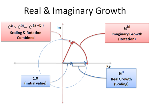
 removed).
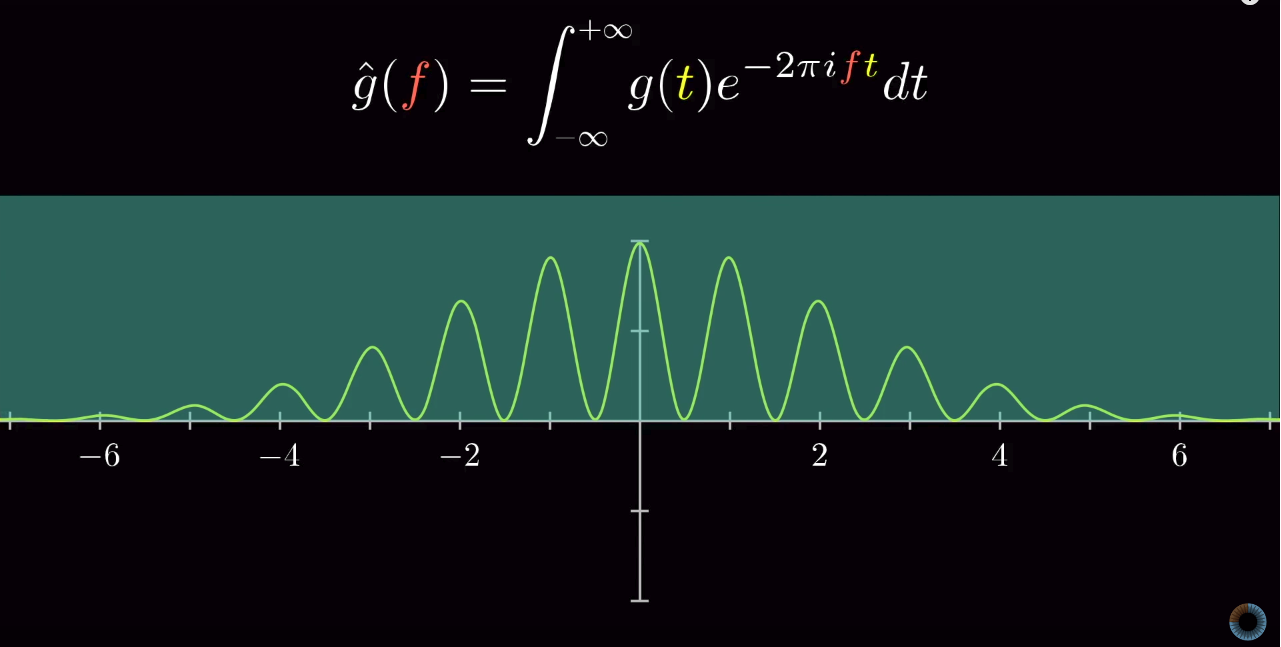
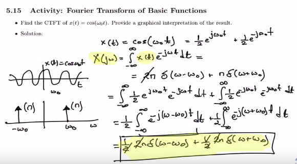
 . The result is two Dirac Delta functions on the frequency domain.
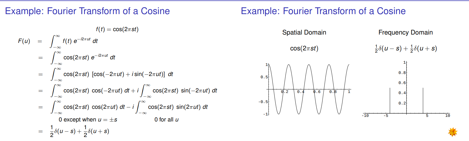
 ,
, 
 does not converge, I have seen many places [15, 18] treating
  . I don’t understand this, but I could think it in an intuitive way: although
  does not converge, its values is confined in a limited range (
 ). Compared to the infinity we obtain from
  , the value of
  . Also, Dirac Delta function is defined as (its proof, which I don’t fully understand, can be found on [11, 12, 13]):

 rather than
  ):
): :
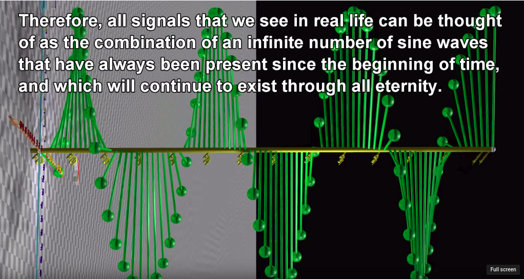
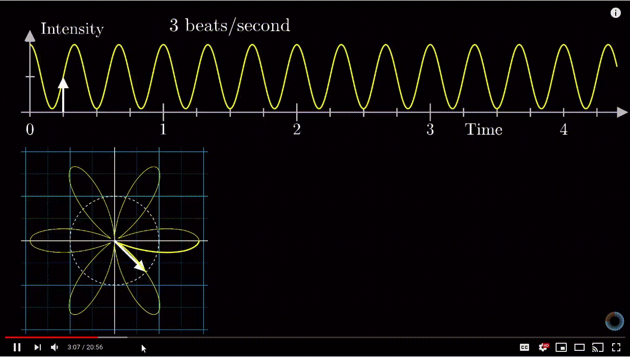
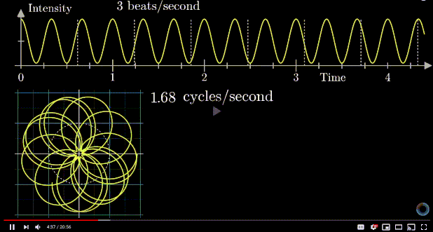
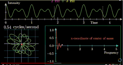
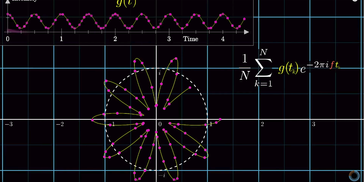
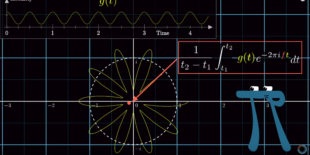
: , then the resultant Fourier transform is the sum of several Dirac functions. That’s how Fourier transform extracts individual signals from the mixed one! And the connection between Euler’s formula and Fourier transform is that the integration required by Fourier transform to obtain the center of mass of the rotation diagram, if connected to Euler’s formula, can be calculated very easily.