Here are some materials I found useful to learn Reinforcement Learning (RL).
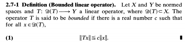
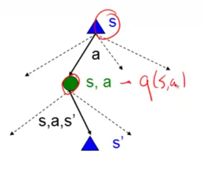
Let’s first look at Markov Decision Process (MDP), in which you know a transition function $latex T(s,a,s’)$ and a reward function $latex R(s,a,s’)$. In the diagram below, the green state is called “q state”.
Some notations that need to be clarified:
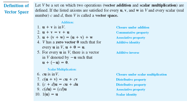
Dynamic programming refers to a collection of algorithms that can be used to compute optimal policies given a perfect model of the environment as a Markov Decision Process (MDP). Before we introduce reinforcement learning, all the algorithms are within the dynamic programming family, such as value iteration, policy evaluation/iteration.
$latex V^*(s)=$expected utility starting in $latex s$ and acting optimally
$latex Q^*(s,a)=$expected utility starting out having taken action $latex a$ from state $latex s$ and thereafter acting optimally
$latex \pi^*(s)=$optimal action from state $latex s$
By definition:
$latex V^*(s)=max_a Q^*(s,a)=max_a \sum\limits_{s’}T(s,a,s’)[R(s,a,s’)+\gamma V^*(s’)] \newline Q^*(s,a)=\sum\limits_{s’}T(s,a,s’)[R(s,a,s’)+\gamma V^*(s’)]$
The second equation is called Bellman Equation. $latex \gamma$ is the discounting factor, meaning that the true value of a state not only depends on the accumulated absolute value of rewards but also on how early we get reward. The earlier we can get reward, the better. Also, if there is no $latex \gamma$, we may have an infinitely large value of a state. If you have $latex N$ states and known $latex T(s,a,s’)$ and $latex R(s,a,s’)$, you can use $latex N$ equations of $latex V^*(s)$ and a non-linear solver to get $latex V^*(s)$. However this may be too complex in practice. Instead, you can learn $latex V^*(s)$ in an iterative way, which is called value iteration:
$latex V_{k+1}^{*}(s) \leftarrow max_a \sum\limits_{s’}T(s,a,s’)[R(s,a,s’)+\gamma V^{*}_k(s’)] $
However note that each iteration takes $latex O(S^2A)$ time, where $latex S$ and $latex A$ are the number of states and actions respectively.
For a given policy $latex \pi$, you can also evaluate the values of states under that policy. In general such process is called policy evaluation:
$latex V^{\pi}(s) \leftarrow \sum\limits_{s’} T(s, \pi(s), s’)[R(s,\pi(s), s’)+\gamma V^{\pi} (s’)] \newline V^{\pi}_{k+1}(s) \leftarrow \sum\limits_{s’} T(s,\pi(s), s’)[R(s,\pi(s), s’)+\gamma V_k^{\pi} (s’)]$
Note that, in policy evaluation of $latex V^{\pi}(s)$, there is no max function in it. In value iteration for $latex V^{*}(s)$, there is max function. For policy evaluation, you can use a linear solver to get $latex V^{\pi}(s)$ (first equation) because there is no max function in the equation. Or you can use value iteration (second equation). If using a small $latex \gamma$, iterative update might be fast because a small $latex \gamma$ usually leads to a quick convergence.
For any given policy $latex \pi$, you can iterate it to find an optimal policy as well as getting $latex V^*(s)$ too. Such process is called policy iteration, which follows two steps:
- fix the current policy $latex \pi_i$, iterate until values converge: $latex V^{\pi_i}_{k+1}(s) \leftarrow \sum\limits_{s’} T(s, \pi_i(s), s’) [R(s, \pi_i(s), s’) + \gamma V^{\pi_i}_k(s’) ]$
- fix the current values, get a better policy by one-step looking ahead: $latex \pi_{i+1}(s)=argmax_a \sum\limits_{s’}T(s,a,s’)[R(s,a,s’)+\gamma V^{\pi_i}_{k+1}(s’)]$.
Value iteration and policy iteration suffer some speed issues in different perspectives. Remember that value iteration on $latex V^{*}(s)$ is slow because each iteration takes $latex O(S^2A)$ time. As comparison, step 1 of policy iteration only considers one action $latex \pi_i(s)$ and related next states $latex s’$. However, you need to wait for all values to converge in step 1 in policy iteration, which also takes time.
All the discussions above happen in the context of MDP. That means, $latex T(s,a,s’)$ and $latex R(s,a,s’)$ are known to you. All the methods we introduced above belong to Dynamic Programming, or called model based methods. Also note that in all these methods, they update estimates on the basis of other estimates. We call this general idea bootstrapping.
In the reinforcement learning we will talk about next, you may not know $latex T(s,a,s’)$ or $latex R(s,a,s’)$. So sometimes they are called model free methods. Many reinforcement learning algorithms also use bootstrapping.
Let’s first talk about a passive reinforcement learning scheme called temporal difference learning. It only estimates $latex V^{\pi}(s)$ for each state given a specific policy $latex \pi$. It is called “passive” reinforcement learning because you are given a fixed policy and you don’t need to learn the optimal policy and only need to evaluate the policy. However, merely knowing $latex V^{\pi}(s)$ does not directly suggest the optimal action for you under the policy $latex \pi$. Thus, there are two kinds of problems all variants of reinforcement learning solve: prediction problem, estimating the value function for a given policy; control problem, finding an optimal policy, the policy maximizing accumulated rewards when traversing through states.
In reinforcement learning, model-free value-iteration and model-free policy-iteration using q-functions are Q-learning and SARSA, respectively [6].
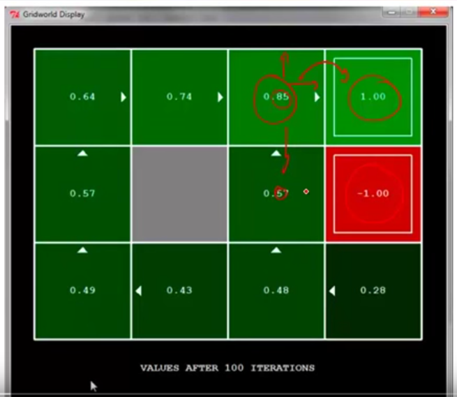
Here is an example using Q learning. Each cell is a state and arrows of all the cells denote a fixed, given policy $latex \pi$. Reward is only given at the top right corner (+1) and the cell below it (-1). We can see after 100 iterations, each cell (state) learns $latex v^{\pi}(s)$. Now, why the cell on the left of +1 cell is 0.85, not 1.00? This is due to the two reasons: 1. the discounting factor $latex \gamma$ makes the $latex V^{\pi}(s)$ approach but never be 1.00; 2. the transition is stochastic. So the transition probability $latex p(s’|s, a)$ is not perfect 1 but could have many possible $latex s’$. For example, at the cell 0.85, even the policy suggests to take right, it has certain chance to go to the cell below, which might lead to the undesirable state. Therefore, this state should not be perfect +1.00.
We can compare to the result of Q-learning, which has the update rule: $latex Q(s,a) \leftarrow (1-\alpha)Q(s,a)+\alpha \cdot [R(s,a,s’) + \gamma max_{a’}Q(s’,a’)]$.
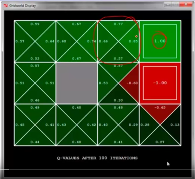
First, note that on the same cell that is on the left of +1 cell, $latex q(s, RIGHT)=0.85$, which is equal to the same cell in the TD learning. This is because the provided policy in TD learning also suggest to take RIGHT. Second, why the cell on the left of -1 cell has $latex q(s, RIGHT)=-0.6$ instead of $latex -0.85$? This is because if an agent stands in the cell, takes RIGHT, but does not land on -1 cell, it will be less likely to get into -1 cell again. However, imagine another agent which stands on the left of +1 cell and takes RIGHT, if he fails to get into +1 cell, he might still stay in the same cell because going UP isn’t really an option, making him ready to get into +1 cell again.
Q-learning is called off-policy learning because what exploration policy does not matter as long as the exploration policy makes you experience all state-action pairs and you set a proper learning rate $latex \alpha$. For example, you are using a very poor exploration policy, and starting from $latex s’$, you take very poor action $latex a’$. However, $latex max_{a’}Q(s’, a’)$ might still be large enough to improve $latex Q(s,a)$. The difference between Q-learning and SARSA, and generally between off-policy and on-policy, can be seen in [4].
An improved Q-learning technique is called Dyna Q-learning, which achieves model learning, direct reinforcement learning and planning (indirect reinforcement learning) in the same algorithm. Model learning means learning a model that produces a prediction of next state and next reward given the current state and an action. In Dyna Q-learning, the model is so trivial – a table recording the last-observed $latex R_{t+1}, S_{t+1}$ for each $latex S_t, A_t$ (Step e). Direct reinforcement learning means the direct update of Q values just as in a normal Q-learning (Step d). Planning means additionally updating Q-values based on simulated experience on the model (Step f).
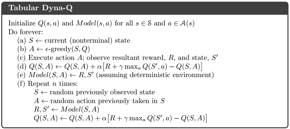
Without planning part, Dyna Q-learning downgrades to a normal Q-learning. The (state-space) planning can be depicted as:
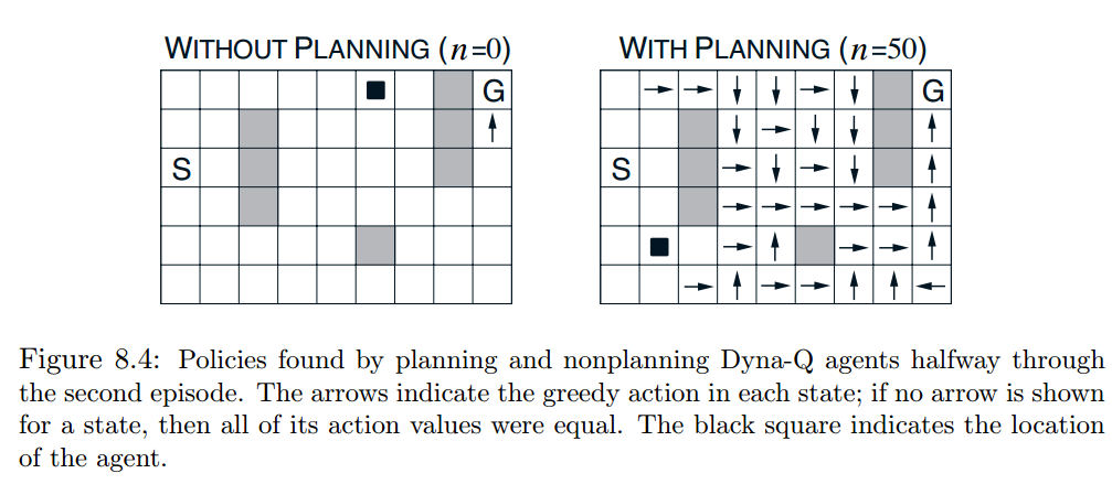
 Because Dyna Q-learning uses additional (simulated) experience to update Q-values, it converges the optimal policy in fewer iterations. Here is an example from Chapter 8.2 in [5].
Currently, I only know Dyna Q-learning is a tabular method, meaning $latex S$, $latex A$ need to be finite, discrete so that we can have an entry for each $latex S, A$ pair.
Now, here is a big roadmap of RL and MDPs:
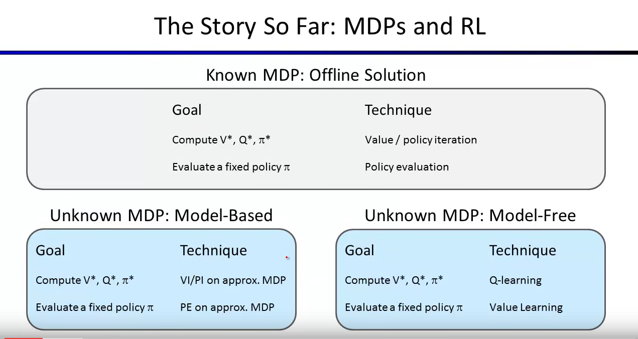
When MDP is known, we can use value iteration and policy iteration to compute $latex V^*$, $latex Q^*$ and $latex \pi^*$. When given a specific policy $latex \pi$, we can evaluate $latex V^{pi}(s)$.
When MDP is unknown, we need to use RL. For model-based learning, we need to build models to estimate $latex T(s,a,s’)$ and $latex R(s,a,s’)$ as an approximated MDP. After that, we can apply value iteration/policy iteration just as on a normal MDP. Similarly we can also do policy evaluation on the approximated MDP.
For model-free learning, we do not need to even know or model $latex T(s,a,s’)$ and $latex R(s,a,s’)$. Nevertheless, we still learn $latex V^*$, $latex Q^*$ and $latex \pi^*$.
The biggest challenge of a naive Q-learning that the size of state action pairs Q(s,a) increases quickly. Therefore, we can generalize state-action by using weights and features describing q states to approximate the learning.
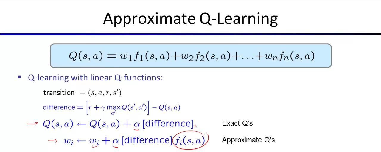 Note in approximate Q-learning, you no longer maintain a table for recording $latex Q(s,a)$. So the only thing you need to do is to update weights.
[1] https://www.youtube.com/watch?v=ggqnxyjaKe4
[2] https://www.youtube.com/watch?v=Csiiv6WGzKM (lecture 8 ~ 11)
[3] http://web.engr.oregonstate.edu/~xfern/classes/cs434/slides/RL-1.pdf
[4] https://czxttkl.com/?p=1850
[5] https://webdocs.cs.ualberta.ca/~sutton/book/bookdraft2016sep.pdf
[6] Reinforcement learning and dynamic programming using function approximators: http://orbi.ulg.ac.be/bitstream/2268/27963/1/book-FA-RL-DP.pdf

 , then we say its augmented cost
  , where
  is a loss function with large values for those deviated state-action pairs and with close-to-zero values for those resembling tutor sequences. Why do we want the augmented cost to be even smaller for those defiant state-action pairs? Because in this way, we make those deviated pairs even harder to be distinguished with the desired pairs. Therefore, we force the algorithm to try hard to update the cost function until it can differentiate augmented costs from different state-action pairs. In other words, the algorithm will learn the cost function such that it differentiates any a desired state-action pair
  with a less desired state-action pair
  by at least a margin
  .
.
 examples, each example is a MDP and a tutor sequence. Different examples may come from different MDPs so this model can learn the cost function generalized to new MDPs which are never seen in the training examples. However, for simplicity, we just assume all training examples are different tutor sequences from the same MDP with state
  and
and  . For simplicity purpose also, an important assumption made throughout [4] is that a tutor sequence is acyclic. This means, any state-action pair is visited at most once in a tutor sequence. Then, it is easy to represent a tutor sequence by
  , a state-action frequency count vector. If the assumption about tutor sequence being acyclic were not made,
  which satisfies certain flow constraints.
 -th example tutor sequence
  . Since we want loss function to be a linear function of
  , we let
  . The more
  should be. A straightforward way to define
  is to make
  , with 0 denoting a particular state-action is visited by both or neither of
  . Now as for cost function, cost function should also factor over states and actions. This means, the cost of a sequence should be the sum of the costs at each state-action pairs visited in the sequence. Suppose we have a feature matrix
  , whose columns are feature vectors at every state-action pair. We also suppose the cost function has a linear weight
  . Then, the cost at one state-action pair is just
  where
where  is the column corresponding to the state-action pair. Finally, the cost of the whole sequence is
  . You can think
  as the accumulated sum of feature vectors on visited state-action pairs.
 .
. . Recall that we want
  ) from tentative paths (arbitrary
  , where
  is all possible sequence in the MDP) by a margin
  . This actually introduces a large number of constraints when
  . Intuitively, this means if
  for each training example. This allows some margin difference constraints to not be satisfied because in real data you may not find a
 resides in both the objective function and the constraints. We want
  . Therefore, we can rewrite our constrained objective function into another non-constrained objective function:
 is a non-differentiable (because of
  ), convex objective. The author in [4] proposes to optimize using subgradient method.
 of a differentiable convex function
  at point
  satisfies:
  . This means the growth of line
  from point
  [7]:
[7]: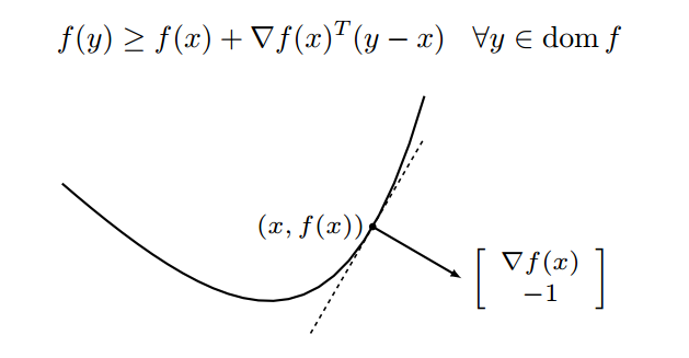
 can be any values such that
  :
: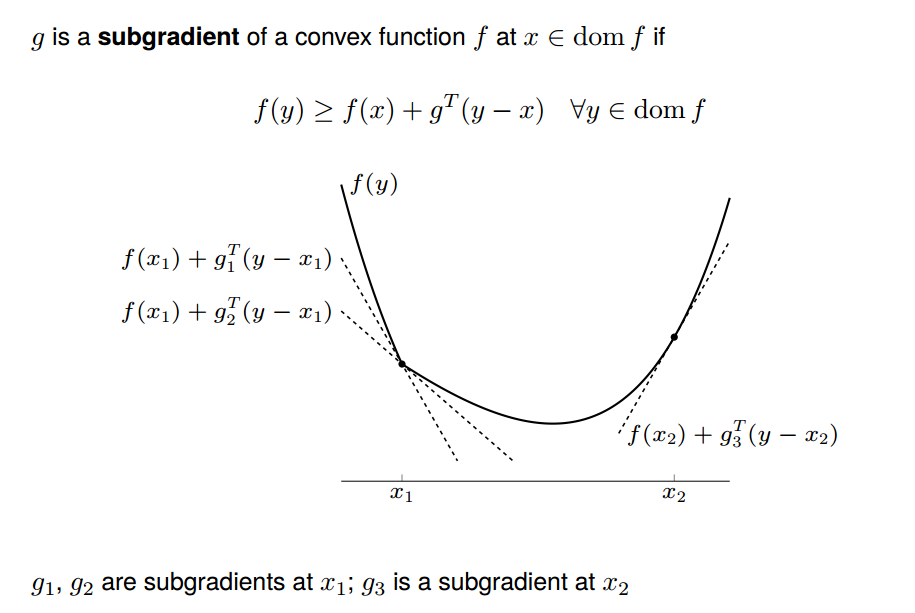
 in
in  . This can be seen as a max over affine functions
  , each shown as dashed line the figure below:
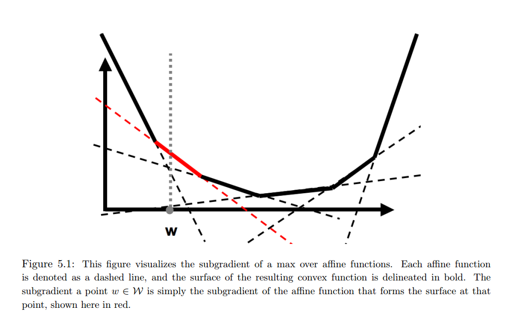

 .
.![w_{t+1} = \mathcal{P}_{\mathcal{W}} [ w_t - \alpha (F(\mu_i - \mu_i^*) + \lambda w_t)] &s=2](https://czxttkl.com/wp-content/ql-cache/quicklatex.com-da1f9da44bb49e5a8b49cb87a57eeaed_l3.png "Rendered by QuickLaTeX.com")
 is projection operator that maps