Traditional Collaborative Filtering
- each user is represented by a O(N) length vector. N is the number of items.
- Therefore, user-item matrix has size O(MN). M is the number of users.
- for a user we want to recommend items for, we scan through user-item matrix, and find most similar k users.
- Based on the item vectors of the most similar k users, we recommend items.
cons: computationally expensive, since you need O(MN) in worst case to find the most similar k users.
Cluster Models
- similarly, construct a user-item matrix of O(MN) size
- cluster users into k groups
- for a user we want to recommend items for, we first identify which cluster he belongs to.
- Among the users in that cluster, we find items to recommend.
pros: for a user to be recommended, only O(k) time is needed to locate his desired cluster, thus reduces time complexity.
cons: The recommendation quality is not too good, given that users in the cluster are not the most similar users to the target user.
Search-Based Method
Search items with same author, artists, categories, etc of the item the target user just bought or rated. Then recommended.
cons: The recommendation quality is still not good, because a user’s next wanted items are not necessarily items with same author, artisits, categories, etc.
Item-to-Item Collaborative Filtering
- each item is represented by a O(M) vector, which records which users have bought this item.
- construct a
 item-item matrix,
  is the similarity between item i and item j. This step runs offline. Worst case time complexity is
  . But since the matrix should be very sparse, and it is computed offline, such time complexity is acceptable.
 - When a target user buys an item, you can immediately find its most similar item and recommend it to the user.
Collaborative filtering in practice often outperforms content based filtering. However, collaborative filtering, either item based or user based, has a drawback: cold start problem. For new products/new user, its vector will not be well represented until a fair amount of time. Therefore,the quality of CF recommendation on the new product/user will downgrade. In light of this, content based filtering has its advantage. Another minor drawback of CF is its inability to recommend to users with unique taste.
Matrix Factorization Model
Each item and user is represented by a vector which describes the item’s or the user’s innate property. The dot product of a user vector ![]() and an item vector
and an item vector ![]() reflects how closely the two relate, where
reflects how closely the two relate, where ![]() , the dimension of the vector, will be determined by how granular you want to model user/item. As in the netflix prize competition, people reported to use 50-1500 dimensions. The higher the dimension they used, the better the recommendation quality reportedly.
, the dimension of the vector, will be determined by how granular you want to model user/item. As in the netflix prize competition, people reported to use 50-1500 dimensions. The higher the dimension they used, the better the recommendation quality reportedly.
The traditional matrix factorization model, such as SVD, can’t directly be applied to factorize user-item matrix because most of its elements are sparse. You can’t just simply zero an entry <i,j> in the user-item matrix.
There are many versions of matrix factorization model.
- In the scenarios where explicit feedbacks are available, we would like to approximate the dot product of
 and
and  to the explicit rating from user u on item i. As given by this paper, the objective function to minimize is:
 where
where  is the real rating from user u to item i.
 - In many other scenarios, only implicit feedbacks are available. For example, each item is a TV show and
 denotes how long user u has watched the show. (unit: minutes). In this case, low
  indicates user u only watched a little portion of the show. But this can be due to many reasons intractable to capture: lack of interest, not perfect time for watching, laptop battery dying, etc. On the other hand, high
  indicates user u showed potentially strong interest in the show. Naturally, we want our objective function to accurately approximate strong
  but relax its rigorousness on approaching weak
  . Therefore, the approximation error,
  , should be weighted by a confidence parameter
  to give higher
  larger importance.
  can take various forms, such as
  or
or  .
. - In implicit feedback scenario, there are two subcategories: ranking based and prediction based, each has its assumption. Ranking based learning algorithm assumes that implicit feedback difference, i.e.,
 , reflects the difference of the user’s interest between item i and j. Prediction based algorithm assumes there is a function
  which binarizes
  which is more or less random/unpredictable/fluctuated. The approximation error thus becomes
  .
.
prediction based paper: http://yifanhu.net/PUB/cf.pdf
ranking based paper: http://wanlab.poly.edu/recsys12/recsys/p83.pdf
Learning for Matrix Factorization Model
Stochastic gradient descent (SGD) or alternating least squares (ALS) can be used to learn parameters in the objective function. SGD is considered easier and faster but ALS can be parallelized on Mapreduce or Sparks. Both SGB and ALS’s time complexity is linear in the size of (user+item). This paper shows different parallelization strategies to learn matrix factorization model.
Bayesian Personalized Ranking Framework
A paper proposes a general Bayesian ranking framework which can be used for various recommendation system algorithm. The idea is to model the probability of observing every pair of items which user prefer differently (through implicit feedback), and maximize the joint probability of observing all such pairs w.r.t model specific parameters. Reading the paper’s section 4.3 will greatly help you understand the whole idea from its listed examples.
Incorporate temporal dynamics in Collaborative Filtering/Matrix Factorization
A more sophisticated model integrates temporal shift of user preference and item property in the recommendation. What they model in temporal aspect includes:
- user rating bias changes over time
- item rating bias (people tend to give higher/lower rating on certain items over others) changes over time
- For matrix factorization models, each component of the user vector (representing the user’s taste in a dimension) changes over time
- For collaborative filtering models, similarity between two items will be affected by time: if ratings for two items (i and j) from the same user happen within short time, their similarity should be high.
Finding candidate items to recommend
Once you have a trained model, the next thing is to give users recommendation. For collaborative filtering, you probably can immediately get most similar items for items a user just bought, depending on how you structure your data. For matrix factor models, you probably need more efforts to find a small set of candidate items, rather than the whole item set, and then determine the recommendation item within the candidate item subset. A stuff at Etcy reported that they used Locality-Similarity Hash (LSH) to find candidates. The item space is divided into subspaces by ![]() planes. Items falling into the same subspace constitute the candidate subsets.
planes. Items falling into the same subspace constitute the candidate subsets.
Restricted Boltzmann Machines for Collaborative Filtering
It originates from a Geoffrey’s paper. (I felt hard to read.) Good tutorial about RBM can be found here: http://blog.echen.me/2011/07/18/introduction-to-restricted-boltzmann-machines/
The basic idea of RBM:
- Input layer is a binary vector of a user of length N, the total size of items. The number of hidden units is parameter and can be tuned.
- Based on the current weights and biases, predict hidden unit values.
- Based on the calculated hidden unit values, recalculate the input layer values
- The difference between the calculated input layer values and the observed input values is the objective function to minimize.
- All users share the same weights and biases.
- After the training process, for a new user with his own item vector, we can see which hidden units are activated hence determine his taste. Then, try to binary his taste at hidden units, and calculate input layer vector. Recommend any activated input unit that the user has not buy the corresponding item.
Deep learning
So far, I’ve only seen deep learning as resorts in content-based recommendation. One guy interned at Spotify reported using Convolutional Neural Network (CNN) on audio signals to extract features in order to contribute to Spotify’s recommendation system. Another guy who worked at Spotify used Recurrent Neural Network (RNN) to predict which track a user will play next. The input to RNN will be user playing track history.
LDA in Recommendation System
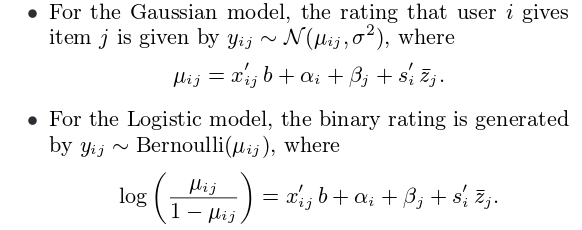
fLDA is a model that borrows ideas from classic LDA model. It is suitable to the cases where meta-data of items are rich. It proposes that:
where ![]() is the user-item interaction vector,
is the user-item interaction vector, ![]() is the weight vector for
is the weight vector for ![]() ,
, ![]() is user
is user ![]() ‘s bias variable,
‘s bias variable, ![]() is item
is item ![]() ‘s bias variable,
‘s bias variable, ![]() is the user’s topic vector on
is the user’s topic vector on ![]() topics (representing the user’s interest on the
topics (representing the user’s interest on the ![]() topics), and
topics), and ![]() is the item’s topic soft clustering label.
is the item’s topic soft clustering label. ![]() ,
, ![]() and
and ![]() are all random variables controlled by some forms of prior.
are all random variables controlled by some forms of prior. ![]() is actually a mean of all words’ topic distribution in item
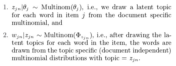
is actually a mean of all words’ topic distribution in item ![]() ‘s meta data. The topic of a word in a item is generated in the following way as the same in classic LDA model:
‘s meta data. The topic of a word in a item is generated in the following way as the same in classic LDA model:
Unlike classic LDA model such that ![]() is purely obtained from Collapsed Gibbs Sampling based upon text data,
is purely obtained from Collapsed Gibbs Sampling based upon text data, ![]() has also interaction with user topic vector
has also interaction with user topic vector ![]() and hence determine his rating
and hence determine his rating ![]() . Therefore, when sampling
. Therefore, when sampling ![]() in the training process (E step), all ratings for the item the word belongs to will take into account:
in the training process (E step), all ratings for the item the word belongs to will take into account:
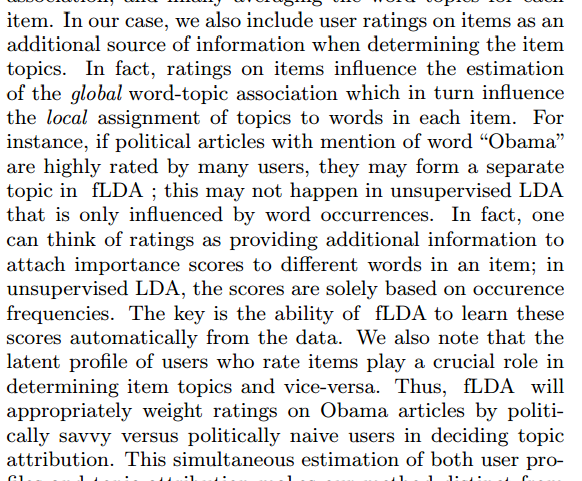
That is why in the paper the authors mentioned that:
The training process is a bit intimidating as shown in the paper. Note that the authors claimed that the training process takes O(# of rating + # or words) time.
Other Tutorial Materials
A very complete recommendation system review tutorial can be found here, which was given by Xaiver Amatrian, previous research director at Netflix and now at Quora. Another tutorial is from Edwin Chen. An overview of content based recommendation approaches is given here. An overview of collaborative filtering methods can be found here. A good slide can be found here.


