Inverse Reinforcement Learning

In my rough understanding, inverse reinforcement learning is a branch of RL research in which people try to perform state-action sequences resembling given tutor sequences.

There are two famous works on inverse reinforcement learning. One is Apprenticeship Learning via Inverse Reinforcement Learning [1], and the other is Maximum Margin Planning [2].

Maximum Margin Planning

In MMP learn a cost function for estimating the cost at each state-action pair. The desired cost function should emit low costs to those state-action pairs appearing in “tutor” sequences (examples) and return high costs to those deviating tutor sequences. If we manage to recover a desired cost function, we can assign the cost for any state-action pair and use path-finding algorithms (e.g., A*, Dijkstra, etc.) to find a sequence on a new environment which has the minimum accumulative sum of costs, that is, a sequence deemed resembling given tutor sequences.

The baisc idea is given in [4]:

Screenshot from 2017-03-29 18:36:37

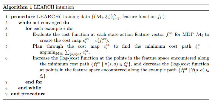
As you see, in line 6, you need to adjust cost function to increase on the current “not-perfect” minimum cost path and decrease the example path. However, you can see that the algorithm doesn’t know how much it should increase the cost for minimum cost path. If one path just deviates from the example path a little bit and another path deviates far more abnormally, how should the adjustment of the cost function reflect that?

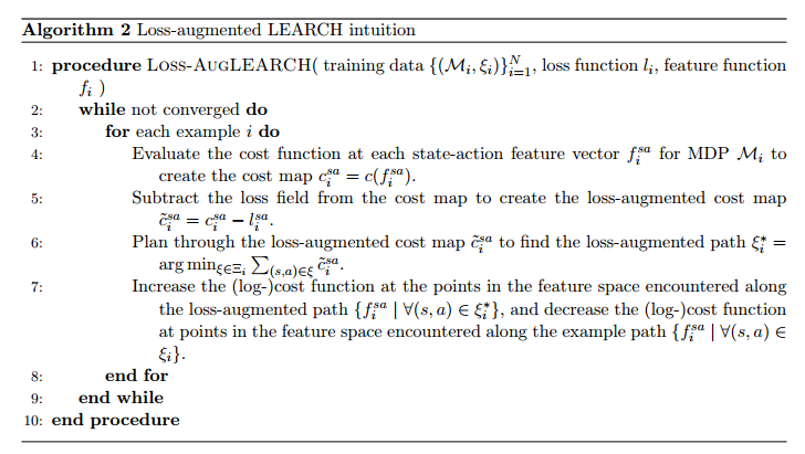
So the author proposes an improvement called “loss augmentation”. Suppose the original cost at a state-action is $c^{sa}$ , then we say its augmented cost $\tilde{c}^{sa} = c^{sa}-l^{sa}$ , where $l^{sa}$ is a loss function with large values for those deviated state-action pairs and with close-to-zero values for those resembling tutor sequences. Why do we want the augmented cost to be even smaller for those defiant state-action pairs? Because in this way, we make those deviated pairs even harder to be distinguished with the desired pairs. Therefore, we force the algorithm to try hard to update the cost function until it can differentiate augmented costs from different state-action pairs. In other words, the algorithm will learn the cost function such that it differentiates any a desired state-action pair $(s,a)$ with a less desired state-action pair $(s',a')$ by at least a margin $l^{s'a'}$ .

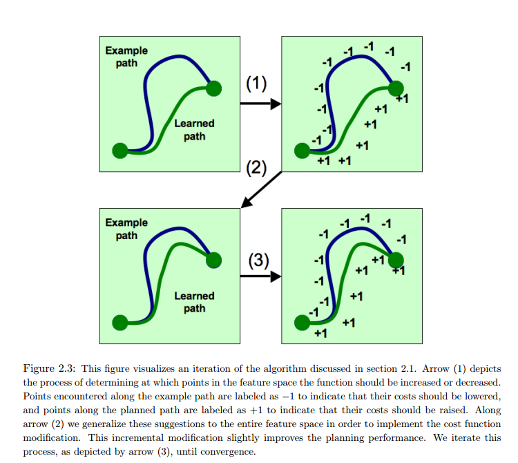
Here is the visualization showing how deviated paths get high rewards (+1) and desired paths get low rewards (-1).

Screenshot from 2017-03-29 21:42:24

And here is the revised algorithm based on Algorithm 1:

Screenshot from 2017-03-29 21:42:30

Now, let’s look at how to learn the cost function using a framework called maximum margin structured classification.

Before that, we introduce preliminaries. In this paper, we are given $N$ examples, each example is a MDP and a tutor sequence. Different examples may come from different MDPs so this model can learn the cost function generalized to new MDPs which are never seen in the training examples. However, for simplicity, we just assume all training examples are different tutor sequences from the same MDP with state $\mathcal{S}$ and $\mathcal{A}$ . For simplicity purpose also, an important assumption made throughout [4] is that a tutor sequence is acyclic. This means, any state-action pair is visited at most once in a tutor sequence. Then, it is easy to represent a tutor sequence by $\mu \in \{0,1\}^{\mathcal{S}\mathcal{A}}$ , a state-action frequency count vector. If the assumption about tutor sequence being acyclic were not made, $\mu \in \mathbb{R}_{+}^{\mathcal{S}\mathcal{A}}$ which satisfies certain flow constraints.

Now remember that the idea is to approximate everything linearly, such as the loss function or the cost function. Each training example has a loss function, which quantifies the difference between an arbitrary sequence and $i$ -th example tutor sequence $\mu_i$ . Since we want loss function to be a linear function of $\mu$ , we let $\mathcal{L}_i(\mu)=l_i^T \mu$ . The more $\mu$ deviates from $\mu_i$ , the higher $\mathcal{L}_i(\mu)$ should be. A straightforward way to define $l_i$ is to make $l_i \in \{0,1\}^{\mathcal{S}\mathcal{A}}$ , with 0 denoting a particular state-action is visited by both or neither of $\mu$ and $\mu_i$ and 1 otherwise. Of course more advanced loss function can be used but the bottom line is to assume $\mathcal{L}_i(\mu) \geq 0$ . Now as for cost function, cost function should also factor over states and actions. This means, the cost of a sequence should be the sum of the costs at each state-action pairs visited in the sequence. Suppose we have a feature matrix $F \in \mathbb{R}^{d \times \mathcal{S} \times \mathcal{A}}$ , whose columns are feature vectors at every state-action pair. We also suppose the cost function has a linear weight $w \in \mathbb{R}^{d}$ . Then, the cost at one state-action pair is just $w^T F_j$ where $F_j$ is the column corresponding to the state-action pair. Finally, the cost of the whole sequence is $w^T F \mu$ . You can think $F \mu$ as the accumulated sum of feature vectors on visited state-action pairs.

Since we assume all training examples come from the same MDP, we can write the data set as $\mathcal{D}=\{(F, \mu_i, l_i)\}^N_{i=1}$ .

Now, the problem is how to obtain $w$ . Recall that we want $w$ to be able to differentiate desired paths ( $\mu_i$ from $\mathcal{D}$ ) from tentative paths (arbitrary $\mu \in \mathcal{G}$ , where $\mathcal{G}$ is all possible sequence in the MDP) by a margin $\mathcal{L}_i(\mu)=l_i^T \mu$ . Therefore, the constraints we would like to impose are: for each $\mu_i$ , for each $\mu \in \mathcal{G}$ , $w^T F \mu_i \leq w^T F \mu - l_i ^T \mu$ . This actually introduces a large number of constraints when $\mathcal{G}$ space is large. Therefore, we reduce the number of constraints by rewriting as: for each $\mu_i$ , $w^T F \mu_i \leq \min\limits_{\mu \in \mathcal{G}} \{w^T F \mu - l_i^T \mu\}$ . Intuitively, this means if $w$ can successfully distinguish $\mu_i$ from the loss-augmented cost of the hardest tentative path $\mu \in \mathcal{G}$ , then it can distinguish from any other tentative paths. Also, we would like to regularize on the norm of $w$ because if $w$ were without norm regularization, it can always scale arbitrarily large to overcome margin difference constraints, voiding the original purpose of adding margins. Moreover, we want to introduce a slack term $\xi_i \geq 0$ for each training example. This allows some margin difference constraints to not be satisfied because in real data you may not find a $w$ which perfectly satisfies all margin difference constraints.

Putting all we describe above, we come to the optimization objective:

$\min\limits_{w \in \mathcal{W}, \xi_i \in \mathbb{R}_+} \frac{1}{N} \sum\limits_{i=1}^N \xi_i + \frac{\lambda}{2} \left\Vert w \right\Vert^2 \newline \forall i, w^T F \mu \leq \min\limits_{\mu \in \mathcal{G}} \{w^T F \mu - l_i^T \mu\} + \xi_i &s=2$

We note that $\xi_i$ resides in both the objective function and the constraints. We want $\xi_i$ as small as possible. Therefore, at the minimizer the slack variables will always exactly equal the constraint violation: $\xi_i = w^T F \mu_i - \min\limits_{\mu \in \mathcal{G}} \{w^T F \mu - l_i^T \mu\}$ . Therefore, we can rewrite our constrained objective function into another non-constrained objective function:

$R(w) = \frac{1}{N} \sum\limits^N_{i=1} \big( w^T F \mu_i - \min\limits_{\mu \in \mathcal{G}} \{w^T F \mu - l_i^T \mu\} \big) + \frac{\lambda}{2} \left\Vert w \right\Vert^2 &s=2$

Now, $R(w)$ is a non-differentiable (because of $\min$ ), convex objective. The author in [4] proposes to optimize using subgradient method.

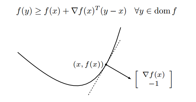
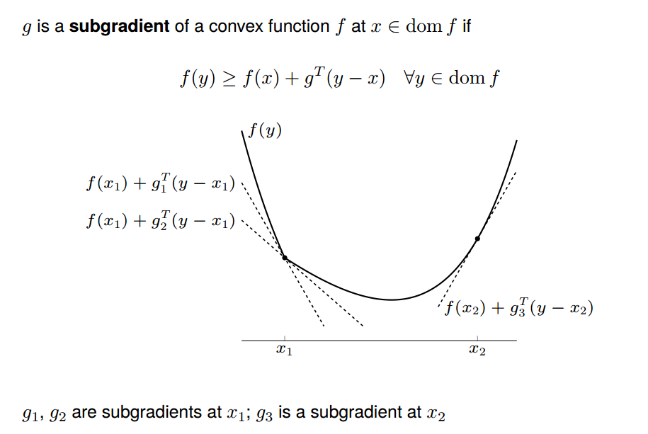
In my mind, subgradient method is really similar to normal gradient descend method. The gradient $\nabla f(x)$ of a differentiable convex function $f(x)$ at point $x$ satisfies: $f(y) \geq f(x) + \nabla f(x)^T (y-x), \forall y \in \text{dom }f$ . This means the growth of line $\nabla f(x)^T (y-x)$ from point $x$ is always equal or slower than $f(y)$ [7]:

Screenshot from 2017-03-30 09:24:17

Subgradient equal to gradient at the part being differentiable. At the non-differentiable part, subgradient $g$ can be any values such that $\{g|g^T(y-x) \leq f(y) - f(x) \}, \forall y \in \text{dom }f$ :

Screenshot from 2017-03-30 09:41:50

Now let’s look at the part $-\min\limits_{\mu \in \mathcal{G}} \{w^T F \mu - l_i^T \mu\}$ in $R(w)$ . This part can be rewritten as $\max\limits_{\mu \in \mathcal{G}} \{-w^T F \mu + l_i^T \mu\}$ . This can be seen as a max over affine functions $\{-w^T F \mu + l_i^T \mu\}, \forall \mu \in \mathcal{G}$ , each shown as dashed line the figure below: Screenshot from 2017-03-30 09:46:16

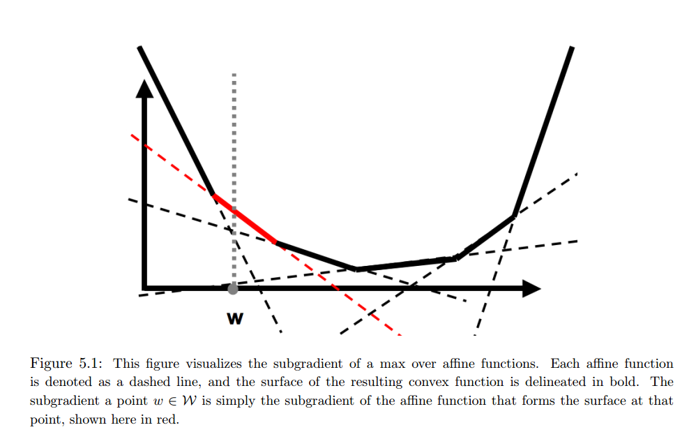
The bold line is $\max\limits_{\mu \in \mathcal{G}} \{-w^T F \mu + l_i^T \mu\}$ . The red line is the subgradient at specific value of $w$ marked by the vertical dashed line. Therefore, the subgradient of $R(w)$ is:

$\nabla R(w) = \frac{1}{N} \sum\limits_{i=1}^N F(\mu_i - \mu_i^*) + \lambda w &s=2$

where $\mu_i^* = argmin_{\mu \in \mathcal{G}} \{w^T F \mu - l_i^T \mu \}$ .

Now, $w$ can be updated online, i.e., being updated after seeing example one by one:

$w_{t+1} = \mathcal{P}_{\mathcal{W}} [ w_t - \alpha (F(\mu_i - \mu_i^*) + \lambda w_t)] &s=2$

where $\mathcal{P}_{\mathcal{W}} ( \cdot)$ is projection operator that maps $w$ to feasible region. For example, sometimes we even require all costs should be positive. How to do projection is something I don’t fully understand in [4]. I hope I will illustrate once I am crystal clear about that.