New progress of generative modeling – flow matching

In a previous post, we discussed an earlier generative modeling called Normalizing Flows [1]. However, Normalizing Flows has its own limitations: (1) it requires the flow mapping function $f(x)$ to be invertible. This limits choices of potential neural network architectures to instantiate $f(x)$ , because being invertible means that hidden layers must have the exact same dimensionality as the input. (2) computing the log⁡ of determinant of the jacobian matrix of $f(x)$ is expensive, usually in $O(N^3)$ time complexity.

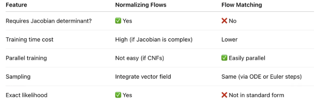
Flow matching is a more recent developed generative modeling technique with lower training cost (see the comparison between Normalizing Flows vs Flow Matching in [2] and a more mathematical introduction of how Flow Matching evolved from Normalizing Flows [6]). In this post, we are going to introduce it. Two materials help me understand flow matching greatly: (1) neurips flow matching tutorial [3] (2) an MIT teaching material [4]

Flow Matching

Motivation

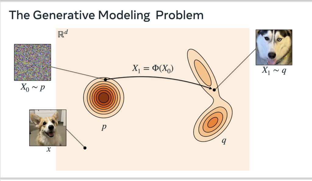
We start from the motivation. Suppose $\mathbb{R}^d$ represents the target space we want to generate (e.g., all dog pictures with $d$ representing the image dimension). The goal of generative modeling is to learn the real target distribution $q$ . To enable generating different targets stochastically, the goal usually becomes to learn the transformation from an initial random distribution $p$ (e.g., Gaussian) the real data distribution $q$ .

A straightforward method is GAN [5]. However, GAN faces various training instability issues and cannot give the likelihood of a data point, while Flow Matching can address both pain points.

Ordinary Differential Equations (ODE)

ODE describes how a system changes over time. An ODE is defined as:

$\begin{align*} \frac{d}{dt} X_t &= \mu_t(X_t) \\ X_0&=x_0, \end{align*}$

where $X: [0, 1] \rightarrow \mathbb{R}^d$ . In natural language, we say that $X_t$ is a variable representing any point in the $d$ -dimensional system at time $t$ , where each dimension is between 0 and 1. At a given time $t$ ( $t$ is also between 0 and 1), $X_t$ should move in the direction of $\mu_t(X_t)$ , which we call the velocity. $\mu_t(X_t)$ is also a $d$ -dimensional vector. The solution of an ODE is called flow, $\psi_t(x_0)$ , which tells you where an initial point will be at time $t$ . Hence $\psi_t(x_0)$ ‘s input is an $d$ -dimensional point and output is also an $d$ -dimensional point. The ODE above can be rewritten with $\psi_t(x_0)$ :

$\begin{align*} \frac{d}{dt} \psi_t(x_0) &= \mu_t(\psi_t(x_0)) \\ \psi_0(x_0)&=x_0, \end{align*}$

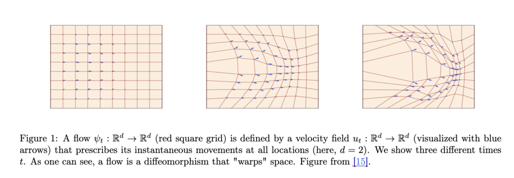
The example below shows how a system moves – the red square grid is the flow, describing each initial point’s “landing” point at time $t$ , and the blue arrow is the velocity at time $t$ .

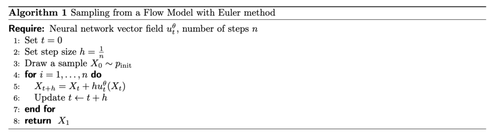
The goal of flow matching is to learn a velocity function $\mu_t^\theta(x)$ such that $X_0 \sim p_{init}$ and $X_1 \sim p_{data}$ . With a known/learned velocity function, you can easily simulate how the system changes, which is equivalent to the flow function $\psi_t(x_0)$ :

Conditional / Marginal Probability Path, Conditional and Marginal Velocity Fields

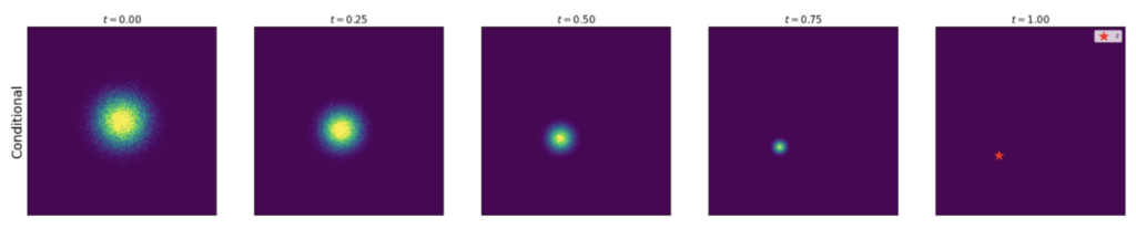
This section is the most mathematical-heavy one. We first introduce the concept of conditional probability path, $p_t(x|z)$ . In natural language, $p_t(x|z)$ means the distribution of the position of a point at time $t$ if that point starts from $p_{init}$ at time 0 and ends at exactly $z$ (i.e., a delta distribution at $z$ ) at time 1, where $z$ is any data sampled from the target distribution $p_{data}$ . 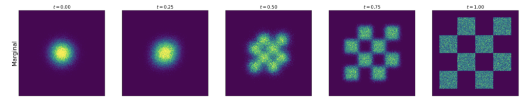Therefore, the marginal probability path $p_t(x)$ can be described as:
$p_t(x)=\int p_t(x|z)p_{data}(z)dz$ .
$p_t(x)$ simply describes the position distribution of the whole system at time $t$ , given the initial distribution is $p_{init}$ and the end distribution is $p_{data}$ .

The diagram below describes an example of conditional probability path $p_t(x|z)$ : it starts from a 2D gaussian distribution and ends at a particular position marked by the red dot.

The diagram below describes an example of marginal probability path $p_t(x)$ : it starts from a 2D gaussian distribution and ends at a chessboard-patterned distribution.

Deriving from the concepts of conditional/marginal probability path, we can also have conditional and marginal velocity field, defined as:
Conditional velocity field: $X_0 \sim p_{init}, X_t\sim p_t(\cdot|z) \; (0 \leq t \leq 1) \Rightarrow \frac{d}{dt} X_t = \mu_t(X_t|z)$
Marginal velocity field: $\mu_t(x) = \int \mu_t(x|z) \frac{p_t(x|z) p_{data}(z)}{p_t(x)} dz$

The formula of marginal velocity field needs a bit work to be proved. We use the rest of this section to prove that.

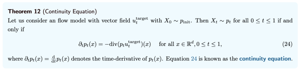
First, we introduce a theorem called Continuity Equation:

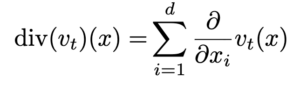
where the divergence operator is defined as:

In natural language, this equation says that the change of marginal probability path w.r.t. time is equal to the negative divergence of $p_t(x) \cdot \mu_t(x)$ . The same theorem can also be applied to the conditional probability path: $\partial_t p_t(x|z) = -div\left(p_t(\cdot|z)\mu_t(\cdot|z)\right)(x)$ .

Now we can show that:

$\begin{align*} \partial_t p_t(x) &= \partial_t \int p_t(x|z)p_{data}(z) dz\\ &=\int \partial_t p_t(x|z)p_{data}(z) dz \\ &=\int -div\left( p_t(\cdot|z)\mu_t(\cdot|z) \right)(x) p_{data}(z) dz \\ &=-div \left( \int p_t(x|z) \mu_t(x|z) p_{data}(z)dz\right)(x) \\ &=-div \left( p_t(x)\int \mu_t(x|z) \frac{p_t(x|z) p_{data}(z)}{p_t(x)}dz\right)(x) \\ &=-div\left( p_t \mu_t \right)(x) \qquad \text{(by definition)} \end{align*}$

By the last two equations, we proved the relationship between the marginal and conditional velocity fields: $\mu_t(x) = \int \mu_t(x|z) \frac{p_t(x|z) p_{data}(z)}{p_t(x)} dz$

Training a Practical Flow Matching model

To reiterate the motivation of flow matching: our goal is to learn a velocity function $\mu_t^\theta(x)$ such that $X_0 \sim p_{init}$ and $X_1 \sim p_{data}$ . Therefore, the ultimate goal should be:
$\mathcal{L}_{FM}(\theta) = \mathbb{E}_{t\sim Unif[0,1], x\sim p_t} \left[ \left\Vert \mu_t^\theta(x)-\mu_t(x) \right\Vert^2 \right] = \mathbb{E}_{t\sim Unif[0,1], z\sim p_{data}, x\sim p_t(\cdot|z)} \left[ \left\Vert \mu_t^\theta(x)-\mu_t(x) \right\Vert^2 \right]$

Recall in the section above that $\mu_t(x) = \int \mu_t(x|z) \frac{p_t(x|z) p_{data}(z)}{p_t(x)} dz$ , which involves an integration operator and thus is intractable. Interestingly, we can prove that $\mathcal{L}_{FM}(\theta)=\mathbb{E}_{t\sim Unif[0,1], z\sim p_{data}, x\sim p_t(\cdot|z)} \left[ \left\Vert \mu_t^\theta(x)-\mu_t(x) \right\Vert^2 \right] = \mathbb{E}_{t\sim Unif[0,1], z\sim p_{data}, x\sim p_t(\cdot|z)} \left[ \left\Vert \mu_t^\theta(x)-\mu_t(x|z) \right\Vert^2 \right] = \mathcal{L}_{CFM}(\theta)$ . Therefore, we can explicitly regress our parameterized velocity function against a tractable conditional vector field. This proof can be found in Theorem 18 in [4].

The exact form of $\mu_t(x|z)$ depends on what family of probability path we choose. One particularly popular probability path is the Gaussian probability path. We can define $\alpha_t$ and $\beta_t$ to be two continuously differentiable, monotonic functions with $\alpha_0=\beta_1=0$ and $\alpha_1=\beta_0=1$ . We can verify that the conditional Gaussian probability path parameterized by $\alpha_t$ and $\beta_t$ , $p_t(\cdot|z)=\mathcal{N}(\alpha_tz, \beta_t^2 I_d)$ , satisfies the definition of a conditional probability path: at time 0, $p_0(\cdot|z) = \mathcal{N}(\alpha_0 z, \beta_0^2 I_d) = \mathcal{N}(0, I_d)$ and $p_1(\cdot|z) = \mathcal{N}(\alpha_1 z, \beta_1^2 I_d) = \delta_z$ . Note that, with the Gaussian conditional probability path, we can simulate the position of $x_t$ : $x_t = \alpha_t z + \beta_t \epsilon$ , where $\epsilon \sim \mathcal{N}(0, I_d)$ . We can then prove that $\mu_t(x|z)=\left(\dot{\alpha_t}-\frac{\dot{\beta_t}}{\beta_t}\alpha_t \right)z + \frac{\dot{\beta_t}}{\beta_t}x$ (see detailed proof in Example 11 in [4]).

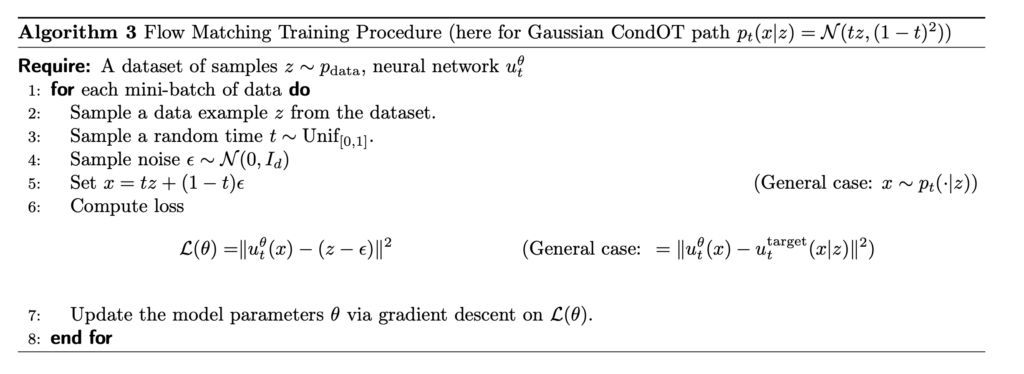
With all these intermediate artifacts, we can derive the loss function:

$\begin{align*} \mathcal{L}_{CFM}(\theta) &= \mathbb{E}_{t\sim Unif[0,1], z\sim p_{data}, x\sim p_t(\cdot|z)} \left[ \left\Vert \mu_t^\theta(x)-\mu_t(x|z) \right\Vert^2 \right] \\ &= \mathbb{E}_{t\sim Unif[0,1], z\sim p_{data}, x\sim p_t(\cdot|z)} \left[ \left\Vert \mu_t^\theta(x)-\left(\dot{\alpha_t}-\frac{\dot{\beta_t}}{\beta_t}\alpha_t \right)z - \frac{\dot{\beta_t}}{\beta_t}x \right\Vert^2 \right] \\ &(\text{let } x=\alpha_t z + \beta_t \epsilon) \\ &= \mathbb{E}_{t\sim Unif[0,1], z\sim p_{data}, x\sim p_t(\cdot|z)} \left[ \left\Vert \mu_t^\theta(\alpha_t z + \beta_t \epsilon) - (\dot{\alpha_t} z + \dot{\beta_t} \epsilon) \right\Vert^2 \right] &(\text{special case: } alpha_t=t, \beta_t=1-t) \\ &=\mathbb{E}_{t\sim Unif[0,1], z\sim p_{data}, x\sim p_t(\cdot|z)} \left[ \left\Vert \mu_t^\theta(tz+(1-t)\epsilon) - (z- \epsilon) \right\Vert^2 \right] \end{align*}$

References

[1] https://czxttkl.com/2021/11/15/normalizing-flows/
[2] https://medium.com/@noraveshfarshad/flow-matching-and-normalizing-flows-49c0b06b2966
[3] https://neurips.cc/virtual/2024/tutorial/99531
[4] https://diffusion.csail.mit.edu/docs/lecture-notes.pdf
[5] https://czxttkl.com/2020/12/24/gan-generative-adversarial-network/
[6] https://mlg.eng.cam.ac.uk/blog/2024/01/20/flow-matching.html