In this post I am going to share my understanding of the paper: Markov Chain Sampling Methods for Dirichlet Process Mixture Models.
In chapter 2, it introduces the basic concept of Dirichlet Process Mixture Models. In (2.1), we have:
$latex y_i | \theta_i \sim F(\theta_i) \newline \theta_i | G \sim G \newline G \sim DP(G_0, \alpha)$
Think the three formulas in an example of a mixture of Gaussian distributions. We have a bunch of data points that we know are from a mixture of Gaussian distributions. Therefore, each data point is from a Gaussian distribution governed by the parameter $latex \theta_i=(\mu_i, \sigma_i)$. That is, $latex P(y_i | \theta_i) = \frac{1}{\sqrt{2\pi\sigma_i^2}}e^{-\frac{(y_i-\mu_i)^2}{2\sigma_i^2}} &s=2$. Multiple data points may belong to the same distribution, i.e., it is possible that $latex \theta_i = \theta_j \text{ for } i \neq j$. However we do not know the number of clusters nor the cluster assignment of the data points yet.
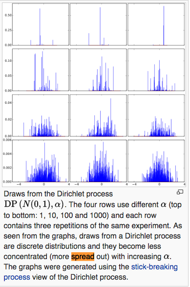
$latex G_0$ is a continuous distribution, let’s say $latex G_0 \sim \mathcal{N}(\mu_0, \sigma_0^2)$. Based on the definition from Dirichlet Process,, $latex G \sim DP(G_0, \alpha)$ is actually a discrete distribution resulting from sampling from $latex G_0$. If $latex \alpha \rightarrow 0$, $latex G$ is more concentrated on a few points. If $latex \alpha \rightarrow \infty$, $latex G$ is widely spread out just as $latex G_0$. (Below is an illustration from Wikipedia)
Consequently, the second formula of 2.1, $latex \theta_i|G \sim G$, says that every data point’s cluster parameter is drawn from the discrete distribution, $latex G$.
Describing formula 2.1 in a generative way, a data point is generated either based on the same cluster parameter of other existing data points, or a new cluster parameter shared by no other data point. The determination of either way depends on whether this data point fits into any existing cluster parameter (how possible the data is generated under any existing cluster parameter) and the popularity of existing cluster parameters (the more data points a cluster parameter is shared by, the more likely it is to be assigned to new data points).
Now, let’s come back to our ultimate goal: you are given a dataset $latex Y=\{y_1, \cdots, y_n\}$. You know $latex Y$ is generated from a dirichlet process mixture model. You do not know $latex \Theta = \{ \theta_1, \cdots, \theta_n \}$ in advance. Your goal is to recover $latex \Theta$.
The joint distribution of $latex \Theta$ is:
$latex p(\Theta | Y, G_0, \alpha) \propto \prod\limits_i P(y_i|\theta_i) \cdot \int P(\theta_i | G) \cdot P(G|G_0, \alpha) dG $
Apparently, the joint distribution is not easy to calculate. But the conditional probability of $latex \theta_i$ given all other parameters $latex \Theta^{-i}$ and $latex Y$ is relatively easy if $latex F(y_i, \theta_i)$ and $latex G_0(\theta_i)$ is conjugate:
$latex \theta_i | \Theta^{-i}, Y \sim \sum\limits_{j \neq i} q_{i,j} \delta(\theta_j) + r_i H_i \newline q_{i,j} = bF(y_i, \theta_j) \newline r_i = b \alpha \int F(y_i, \theta) dG_0(\theta) \newline b = \text{normalization constant} &s=2$
The above is actually from formula 3.2~3.4 in the paper. To clarify, we skip explaining formula 2.2 as it is the probability $latex \theta_i$ conditional only on $latex \Theta^{-i}$ but not including $latex Y$.
The problem of formula 3.2 is that in real world dataset, many data points share the same cluster parameters. Let’s say there are five data points, $latex y_1, y_3, y_6, y_7, y_8$ actually share the same $latex \theta$. As a result, to sample $latex \theta_1, \theta_3, \theta_6, \theta_7, \theta_8$ to simultaneously converge to the same value will take very long time. Therefore, the paper gives Algorithm 2 which determines every cluster’s $latex \theta$ (instead of every data point’s $latex \theta_i$) after cluster assignments of all data points are sampled.
Algorithm 2 is based on another perspective (formula 2.3) to understand Dirichlet Process Mixture Models. Describing formula 2.3 in a generative way, you can say that each data point is generated by first choosing whether it belongs to an existing cluster or form a new cluster itself. Its value is then generated by the parameter of the chosen cluster. Another thought helpful for understanding is to think that whether a data point is generated from a cluster depending on both the cluster popularity and its likelihood within the cluster.
Ok. The above is just the basic concept part of the paper. The paper introduces more advanced sampling algorithms (Metropolis-Hastings) when prior is not conjugate. But using not conjugate prior is really rare in my research, at least for now. So I will just stop here.
The Dirichlet Process Mixture Model is applied in a recommendation system paper: CoBaFi – Collaborative Bayesian Filtering. In this paper, user/item latent factors are assumed to be from a mixture of Gaussians although we do not know the number of clusters in advance. This is very intuitive, since many users and items in real world tend to form similar populations. Advanced users, with sophisticated browsing data, could form their own small clusters. Casual users, with sparse but similar browsing data, can be easily grouped together. After grouping users and items, cluster parameters can be estimated more reliably compared to users/items parameters estimated individually.
Another interesting point of the recommendation paper is their finding that ratings $latex \{r_{ij}\}$ are often not following normal distribution while the paper still assumes all user/item clusters are gaussian distributed and cluster parameters are from a Gauss-Wishart distribution. Due to the non-conjugacy, the paper chooses to use Metropolis-Hastings sampling algorithm.
Reference:
http://www.stat.ufl.edu/archived/casella/OlderPapers/ExpGibbs.pdf