czxttkl

Andrew Ng Tutorial: https://web.stanford.edu/class/cs294a/sparseAutoencoder_2011new.pdf

UFLDL Exercise: http://ufldl.stanford.edu/wiki/index.php/Exercise:Sparse_Autoencoder

A Chinese blog: http://www.cnblogs.com/tornadomeet/archive/2013/03/20/2970724.html

Stacked Denoising Autoencoder (paper): http://jmlr.csail.mit.edu/papers/volume11/vincent10a/vincent10a.pdf

I am going to demonstrate a simple version of convolutional neural network, a type of deep learning structure in this post. 

Motivation

Knowing normal multi-layer neural network (probably the one with input layer, output layer and one hidden layer) is helpful before you proceed reading this post. A good tutorial of MLN can be found here:  http://neuralnetworksanddeeplearning.com/index.html

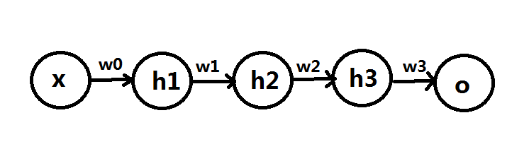
As you can see from the figure above, which shows a typical structure of MLN, all input units are connected to all hidden units. Output units are also fully connected to hidden units.  Such structure suffers some drawbacks in certain contexts. For example, the size of weights to be learnt can be huge to pose challenge to memory and computation speed. ($latex N_{input} \times N_{hidden} \times N_{output}$). Moreover,  after such structure completes its training process and is applied on test data, the learnt weights may not work well for those test data with similar contents but small transformation variance. (e.g. a little horizontal movement of a digit in a image is recognized as the same digit in essence. However the area where the movement happened before and after may correspond to different weights thus the structure becomes more error prone.) Convolutional Neural Network (CNN) is designed as a structure where there exists fewer number of weights that can be shared across different regions of input. A simple pedogogical diagram showing a basic structure of CNN can be seen below (left). The structure on the right below is normal MLN structure with fully connected weights.

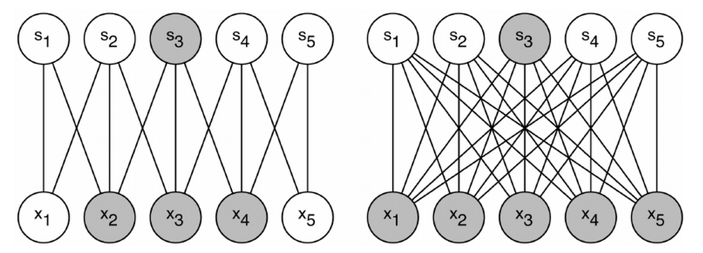
Let’s look at an example (on the left). Every hidden unit ($latex s_1, s_2, \cdots, s_5$) connects with only three input units with exactly same three weights.  For example, the shaded hidden unit $latex s_3$ connects with $latex x_2, x_3 \text{ and } x_4$ just as $latex s_4$ does with $latex x_3, x_4 \text{ and } x_5$. On the contrary, if $latex s_3$ was a hidden layer in MLN, it would connect to all the input units as the right diagram shows. A group of shared weights are called kernel, or filter. A practical convolution layer usually has more than one kernel.

 

Why “Convolution”?

The example we just showed has only one dimension input units. Images, however, are often represented as a 2-D array. If the input in a deep learning network structure is two dimensional, we should also choose 2-D kernels that connect local areas in 2-D inputs. In the computer vision area, the affine transformation of 2-D input passing through a 2-D kernel can be calculated in an operation called convolution.  A convolution operation will first rotate the kernel 180 degrees and then element-wisely multiply the rotated kernel with the input. An example is shown below:

In the output, 26 = 1*5 + 2*4 + 4*2 + 5*1; 38 = 2*5 + 3*4 + 5*2 + 6*1; 44=4*5 + 5*4 + 1*2 + 2*1; 56 = 5*5 + 6*4 + 2*2 + 3*1.

Since the convolution operation is usually implemented efficiently to compute element-wise multiplication of input and kernel, hence the name “convolutional neural network”. When we compute element-wise multiplication of a kernel and an input in CNN, we need to first rotate 180 degrees of the kernel and then apply the convolution operation, since what we want is the element-wise multiplication of the input and the kernel itself rather than its rotated counterpart. In fact, the element-wise multiplication without rotating kernel in the first place has also a corresponding operation in computer vision, which is called “correlation“. More information about convolution and correlation can be found here: http://www.cs.umd.edu/~djacobs/CMSC426/Convolution.pdf 

 

Structure

In this chapter, a simple version of CNN, already implemented by myself, is shown below. 

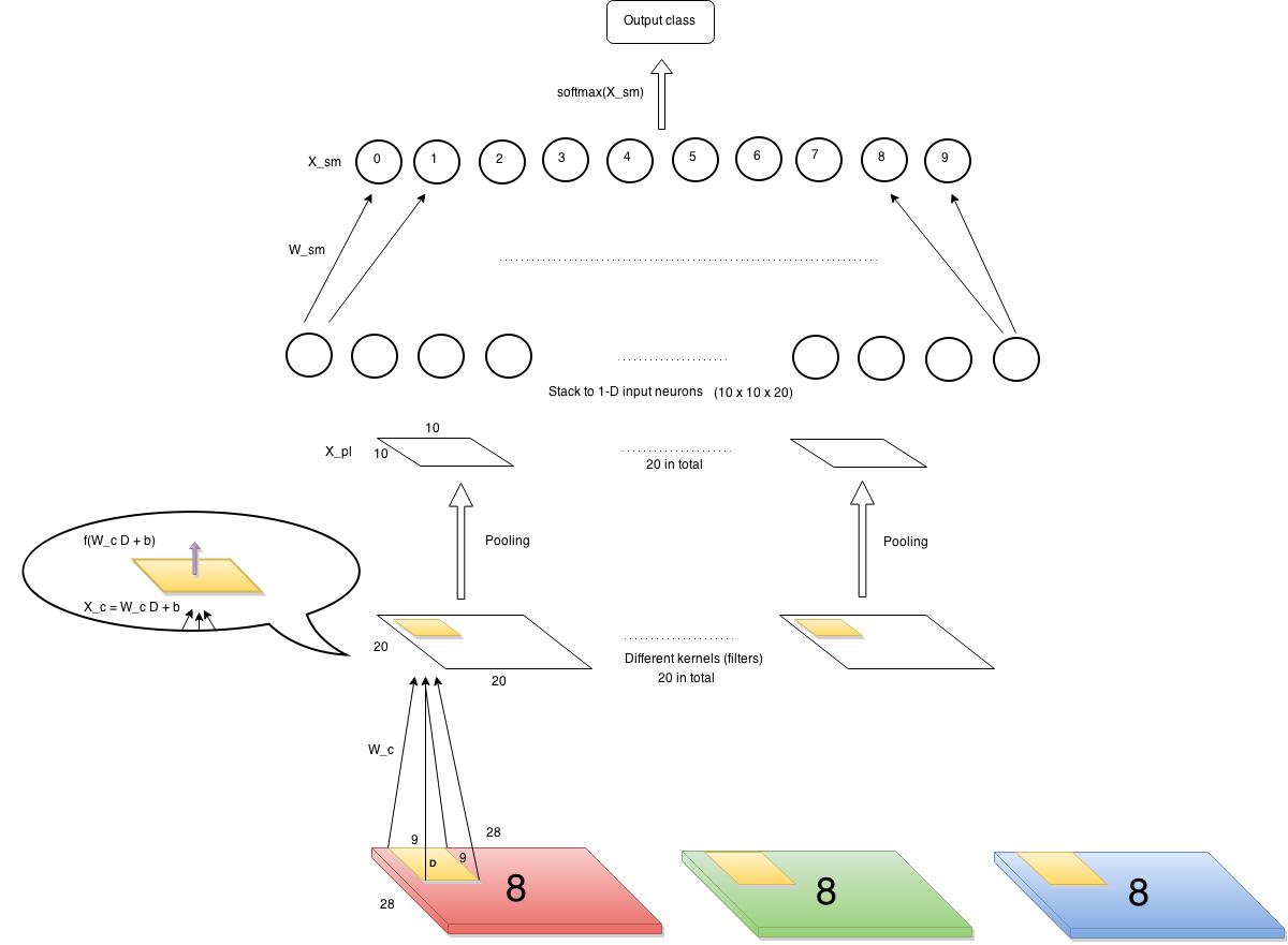
Let’s first define our input and output. The input is images of 28×28 pixels each containing a single digit. The images have several channels (RGB, e.g.)  But in our example, we choose to use only one channel, say, red channel. There will be ten output classes corresponding to 0~9 digits. So the data points can be represented as $latex (\bf{X_1}, y_1)$, $latex (\bf{X_2}, y_2)$, $latex \cdots$, $latex (\bf{X_n}, y_n)$, where $latex \bf{X_i} \in \mathbb{R}^{28\times28}$ and $latex y_i$ is a label among 0~9.

First layer (from bottom) is a convolution layer. We have 20 kernels, each is 9 x 9 (i.e., each kernel connects to a 9×9 pixels in input images each time). Each cell in the convolution layer is an output of a non-linear activation function which takes as input affine transformation of the corresponding area in input images. As you can see from the diagram above, a kernel with weights $latex W_c$ is shown here. $latex W_c \in R^{9\times9}$. The value of each cell in the convolution layer is $latex f(W_c D + b)$, where $latex D$ is the corresponding area in input, and the function $latex f$ in our case is a sigmoid function.

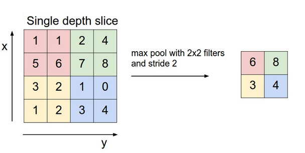
The next layer is a pooling layer, which extracts only partial cell values from the convolution layer and feeds into next layer. It often has two types, max pooling layer and mean pooling layer. It greatly reduces the size of previous layer at risk of losing information, which we assume is not too important thus can be discarded. The chart below gives an example of how a max pooling layer with $latex 2\times 2$ kernels and stride 2 works. In our CNN example, we also decide to use such max pooling layer, which results in $latex 10 \times 10$ pooling output each.

The last layer is softmax layer. Before continuing, it is mandatory to understand how softmax layer works. A good tutorial can be found here: http://ufldl.stanford.edu/tutorial/supervised/SoftmaxRegression/. Softmax layer only takes one dimension input therefore we need to horizontally stack all the outputs from the previous layer (pooling layer). Since we have twenty kernels in the convolution layer, we have 20 pooling results in the pooling layer, each of size $latex 10 \times 10$. So the stacked input is a vector of 2000 length. 

 

Cost function

The cost function which gauges the error thus needs to be minimized is:

$latex C=-\frac{1}{n}\sum\limits_{i=1}^n e(y_i)^T \log(P_{softmax}(X_i)) + \lambda (\left\Vert W_c \right\Vert^2 + \left\Vert W_{sm} \right\Vert^2)&s=2$

 How to understand this cost function?

$latex \log(P_{softmax}(X_i))$ (a vector of length 10) is the log probabilities of $latex X_i$ belonging to the ten classes. You can find more information about softmax here. $latex e(y_i)$ is a one-hot column vector with only one component equal to 1 (residing at $latex y_i$-th component) and otherwise 0. For example, if the label $latex y_i$ of a data point is 8, then $latex e(y_i) = (0,0,0,0,0,0,0,0,1,0)$, each component corresponding to 0~9 digit labels.  For a specific data point $latex (\bf{X_i}, y_i)$, $latex e(y_i)^T \log(P_{softmax}(X_i))$ returns a scalar which is the log probability of $latex X_i$ belonging to the true class. Of course we want this scalar to be as large as possible for every data point. In other words, we want the negative probability as small as possible. That’s all $latex -\frac{1}{n}\sum\limits_{i=1}^n e(y_i)^T \log(P_{softmax}(X_i)) &s=2$ says!

The second part of the cost function is a regularization term where $latex \lambda$ is a weight decay factor controlling the $latex L_2$ norms of weights of the convolution layer and the softmax layer. 

 

Backpropagation

The backpropagation process usually goes like this:

1. Calculate $latex \delta_l = \frac{\partial C}{\partial X_l} &s=2$, dubbed “sensitivity“, which is the partial derivative of the cost function regarding to the input of the last function in the  layer $latex l$. For example, in a convolution layer, the last function is a sigmoid activation function. So the sensitivity of the convolution layer would be the partial derivative of $latex C$ regarding the input of the sigmoid function. See $latex X_c$ in the bubble in the structure diagram above or below. For another example, the last function in a softmax layer is normalization in exponential forms: $latex \frac{exp(W_{sm}(i,:)X)}{\sum_{j=1}^{10}exp(W_{sm}(j,:)X)} &s=2$ for integer $latex i \in [0,9]$. ($latex X$ is the output from the previous layer.) Thus, the sensitivity of the softmax layer is the derivative of the cost function w.r.t  $latex X_{sm} = W_{sm}X$.
2. Calculate $latex \frac{\partial C}{\partial W_l} = \frac{\partial C}{\partial X_l} \cdot \frac{\partial X_l}{\partial W_l} &s=2$, where $latex \frac{\partial C}{\partial X_l} &s=2$ is the sensitivity calculated in the step 1.
3. Update $latex W_l$ by $latex W_l = W_l – \alpha \frac{\partial C}{\partial W_l} &s=2$

We again put the structure diagram here for you to view more easily.

First we start to examine $latex \delta_{softmax} = \frac{\partial C}{\partial X_{sm}} &s=2$. Note where $latex X_{sm}$ is in the structure diagram. According to the derivations here , we can know that $latex \delta_{softmax} = – (e(y) – P_{softmax}(X_{i}))&s=2$, where $latex e(y)$ is an all-zero-but-one-one vector as we mentioned before.

Second, we examine the sensitivity of the pooling layer: $latex \delta_{pooling} = \frac{\partial C}{\partial X_{pl}} = \frac{\partial C}{\partial X_{sm}} \cdot \frac{\partial X_{sm}}{\partial X_{pl}} &s=2$. Since the pooling layer is simply a size-reduction layer you would find that $latex \frac{\partial X_{sm}}{\partial X_{pl}}$ is just $latex W_{sm}$. Therefore $latex \delta_{pooling}$ can be efficiently computed by matrix multiplication of $latex \delta_{softmax}$ and $latex W_{sm}$. After this step, an additional unsampling step is needed to restore the sensitivity to the size consistent with the previous layer’s output. The #1 rule is to make sure the unsampled layer has the same sum of sensitivity distributed in a larger size. We show the examples of unsampling in a mean pooling layer and a max pooling layer respectively. In the max pooling, sensitivity is unsampled to the cell which had the max value in the feedforward. In the mean pooling, sensitivity is unsampled evenly to the local pooling region.

 

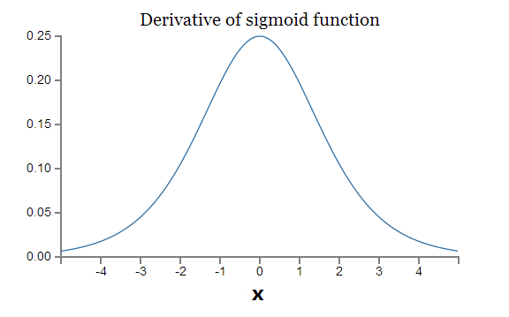
Lastly, the sensitivity of the convolution layer is $latex \delta_{c} = \frac{\partial C}{\partial X_{pl}} \cdot \frac{\partial X^{unsampled}_{pl}}{\partial X_c} &s=2$. Note that $latex \frac{\partial X^{unsampled}_{pl}}{\partial X_c} &s=2$ is the derivative of the sigmoid function, which is $latex f(X_c)(1-f(X_c)$. 

 

Update weights

Updating softmax layer is exactly the same as in a normal MLN. The pooling layer doesn’t have weights to update. Since a weight in a filter in a convolution layer is shared across multiple areas in the input, so the partial derivative of the cost function w.r.t to a weight needs to sum up the element-wise product of the sensitivities of the convolution layer and input. Again you can use the convolution operation to achieve this.

 

My code  

I implemented a simple verison of  CNN and uploaded to PYPI. It is written in Python 2.7. You can use `pip install SimpleCNN` to install it. The package is guaranteed to work under Ubuntu. Here is the code (See README before use it): CNN.tar

 

References  (In a recommended reading order. I read the following materials in this order and found understanding CNN without too much difficulty.)

Deep learning Book (In preparation, MIT Press):

http://www-labs.iro.umontreal.ca/~bengioy/DLbook/convnets.html

Lecunn’s original paper:

http://yann.lecun.com/exdb/publis/pdf/lecun-01a.pdf

Standford Convolutional Networks Course:

http://cs231n.github.io/convolutional-networks 

When you start implementing CNN, this should be a good reference (in Chinese):

http://www.cnblogs.com/tornadomeet/p/3468450.html

 

 

Background

This post reviews how we update weights using the back propagation approach in a neural network. The goal of the review is to illustrate a notorious phenomenon in training MLNN, called “gradient vanish”.

Start

Let’s suppose that we have a very simple NN structure, with only one unit in each hidden layer, input layer and output layer. Each unit has sigmoid function as its activation function:

Also suppose we have training data: $latex (x_1, y_1), (x_2, y_2), \cdots, (x_n, y_n)$. Therefore, we have $latex h_1 = \frac{1}{1+e^{-w_0x_i}}$, $latex h_2 = \frac{1}{1+e^{-w_1h_1}}$, $latex h_3 = \frac{1}{1+e^{-w_2h_2}} $, $latex o = \frac{1}{1+e^{-w_3h_3}}$

Our cost function, which we want to minimize, is as follows:

$latex C=\sum\limits_{i=1}^n \left\Vert y_i – o_i\right\Vert^2$ 

 

If we are going to update $latex w_0$ after a round of inputting all the training data, we use the following rule (with $latex \epsilon$ as the learning rate):

$latex w_0 – \epsilon\nabla_{w_0}C$. 

Due to the chain rule of derivatives, we can have equivalently:

$latex \nabla_{w_0}C = \sum\limits_{i=1}^n\frac{\partial C_x}{\partial o} \cdot \frac{\partial o}{\partial h_3} \cdot \frac{\partial h_3}{\partial h_2} \cdot \frac{\partial h_2}{\partial h_1} \cdot \frac{\partial h_1}{\partial w_0}&s=3$

$latex =\sum\limits_{i=1}^n2(y_i – o_i) \cdot \delta'(w_3h_3) \cdot (-w_3) \delta'(w_2h_2) \cdot(-w_2) \cdot \delta'(w_1h_1) \cdot (-w_1) \cdot \delta'(w_0x_i) \cdot (-x_i)$

$latex =\sum\limits_{i=1}^n2(y_i – o_i)\cdot (-w_3) \cdot (-w_2) \cdot (-w_1) \cdot (-w_0) \cdot (-x_i) \cdot \delta'(w_3h_3) \cdot\delta'(w_2h_2) \cdot\delta'(w_1h_1)\cdot \delta'(w_0x_i)$

,where $latex \delta'(t) = (\frac{1}{1+e^{-t}})’$ is the derivative of sigmoid function.

 

We should be very familiar with the shape of sigmoid function as well as its derivative.

From the two plots above, we know that the largest derivative of sigmoid function is 0.25 and it takes place at x=0. Let’s go back to $latex \nabla_{w_0}C$ of the multiple-layer neural network,  which is the gradient descent of the weight associated with the layer farthest away from the output unit. It has four sigmoid derivatives, namely $latex \delta'(w_3h_3) \cdot\delta'(w_2h_2) \cdot\delta'(w_1h_1)\cdot \delta'(w_0x_i)$, each of which cannot overseed 0.25. As a result, $latex \nabla_{w_0}C$ would become very tiny.

That’s how gradient vanishing happens! It’s the phenomenon that certain weights in a multi-layer neural network cannot get updated effectively. 

 

Reference

http://neuralnetworksanddeeplearning.com/chap5.html

http://www-labs.iro.umontreal.ca/~bengioy/dlbook/mlp.html