czxttkl

I’ve talked about the vanishing gradient problem in one old post in normal multiple layer neural networks. Pascanur et al. (the first in References below) particularly discussed the vanishing gradient problem as well as another type of gradient instable issue, the exploding gradient problem in the scope of recurrent neural network.  

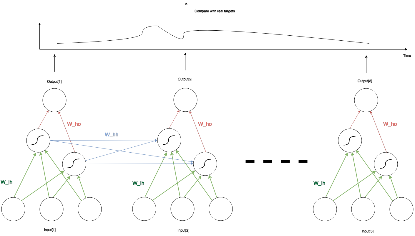
Let’s recap the basic idea of RNN. Here is the sketch of a simple RNN with three inputs, two hidden units and one output. In any given time, the network structure is the same: three input units connect to two hidden units through $latex W_{ih}$ (green lines in the pic), whereas the two hidden units connect to one output through $latex W_{ho}$ (red lines). Between two adjacent time steps, the two hidden units from the earlier network also connect to the two in the later network through $latex W_{hh}$ (blue lines). The two hidden units also perform an activation function. In our case we set the activation function to the sigmoid function. However, the outputs are just linear combination of the hidden unit values.

Pascanur pointed out that, if the weights $latex W_{hh}$ has no singular value larger than the largest possible value of  the differentiation of the activation function of the hidden unit (in our case the sigmoid’s largest differentiation is 0.25), then the RNN suffers from the vanishing gradient problem (i.e., the much more earlier inputs tend to barely have influence on the later outputs). On the other hand, the largest singular value of $latex W_{hh}$ being larger than 0.25 is a necessary condition of the exploding gradient problem: the error of the output regarding the earlier input may augment to a exploding level so that the training never converges.

 Purely by my curiosity, I did some experiments trying to replicate the vanishing gradient problem and the exploding gradient problem. Here are my steps:

1. Initialize an RNN with three inputs, two hidden units and an output unit. The weights connecting them are crafted to let $latex W_{hh}$ have singular values tending to cause either the vanishing gradient problem or the exploding gradient problem. I will record the values of $latex W_{ih}$, $latex W_{hh}$ and $latex W_{ho}$. 
2. Randomly generate input sequences and feed into the RNN in step 1. Record the outputs of the inputs passing through the RNN. The inputs are generated in several sets. Each set has 500 input sequences. But different sets have different lengths of sequences. Doing so lets me examine how the vanishing (exploding) gradient problem forms regarding to the length of sequences.
3. Now start to train a new RNN, with the input and output in step 2.
4. Compare the weights from the two RNNs and see the training is successful (i.e. the weights are close)

Bear in mind that the largest singular value of $latex W_{hh}$ being larger than 0.25 is just a necessary condition of the exploding gradient problem. But I still keep going to see what will happen. The tables below contain the costs after certain epochs given certain lengths of sequences.

When

epoch\seq length	2	10	100
500	1.2e-5	1.44e-5	1.35e-5
1500	3.21e-9	5.11e-9	2.7e-9

 

When 

epoch\seq length	2	10	100
500	0.00144	0.00358	0.0045
1500	2.39e-5	0.00352	0.0045

From the results above, I find that the vanishing gradient problem is hard to replicate (all the costs in the first table converged to small values), as opposed to the exploding gradient problem which emerged given sequences of length 100 (as you can see the costs stuck at 0.0045).

Code

rnn_generator.py: used to generate simulated input and output data passing by fixed weights

import numpy as np
import theano
import theano.tensor as tt

class RNNGenerator(object):
    '''
    Generate a simulated RNN with a fixed set of weights, 
    based on a fixed seed: np.random.seed(19910715)
    Also check out RNNGenerator1, which generates simulated 
    RNN sequences of output with a fixed delay w.r.t input.
    '''
    
    def __init__(self, input_num, output_num, hidden_num):
        np.random.seed(19910715)
        self.input_num = input_num
        self.output_num = output_num
        self.hidden_num = hidden_num
        
        # Initialize weights
        self.W_hh = np.random.randn(hidden_num, hidden_num)
        u, s, v = np.linalg.svd(self.W_hh, full_matrices=True, compute_uv=True)
        s = np.diag(s)
        print u, "\n\n", s, "\n\n", v, "\n"
        print "Close?", np.allclose(self.W_hh, np.dot(np.dot(u, s), v)), "\n"
        
        # Manually craft the largest singular value of W_hh as you wish
        # s[0,0] = 10
        # self.W_hh = np.dot(np.dot(u, s), v)

        self.b_hh = np.random.randn(hidden_num)
        self.W_hi = np.random.randn(hidden_num, input_num)
        
        self.W_yh = np.random.randn(output_num, hidden_num)
        self.b_yh = np.random.randn(output_num)
        
        self.u, self.s, self.v = u, s, v
        
        # Initialize output function
        # Create symbols
        self.W_hh_sym = theano.shared(self.W_hh)
        self.W_hi_sym = theano.shared(self.W_hi)  # hidden_num x input_num
        self.b_hh_sym = theano.shared(self.b_hh)
        inputs_sym = tt.matrix("inputs_sym")  # data_num x input_num
        
        # fn: a lambda expression to define a recurrent process
        # sequences (if any), prior result(s) (if needed), non-sequences (if any)
        outputs_sym, _ = theano.scan(fn=lambda inputs, prior_hidden, W_hh, W_hi, b_hh:
                                     tt.nnet.sigmoid(tt.dot(W_hh, prior_hidden) + tt.dot(W_hi, inputs) + b_hh),
                                     sequences=inputs_sym,
                                     non_sequences=[self.W_hh_sym, self.W_hi_sym, self.b_hh_sym],
                                     # outputs_info is the initial state of prior_hidden
                                     outputs_info=tt.zeros_like(self.b_hh_sym))        
 
        # Doesn't need to update any shared variables, so set updates to None
        self.output_func = theano.function(inputs=[inputs_sym], outputs=outputs_sym, updates=None)
    
    def weights(self):
        return self.W_hh, self.W_hi, self.W_yh, self.b_hh, self.b_yh    
    
    def inputs_outputs(self, data_num, seq_len):
        m_inputs = np.random.randn(data_num, seq_len, self.input_num)
        m_final_outputs = np.zeros((data_num, seq_len, self.output_num))
        for j in xrange(data_num):
            m_hidden = self.output_func(m_inputs[j, :, :])
            m_outputs = np.zeros((seq_len, self.output_num))
            for i in xrange(m_hidden.shape[0]):
                m_outputs[i] = np.dot(self.W_yh, m_hidden[i]) + self.b_yh 
            m_final_outputs[j, :, :] = m_outputs
        
        return m_inputs, m_final_outputs
    
if __name__ == '__main__':
   input_num = 3
   output_num = 1
   hidden_num = 2
   # How delayed outputs will rely on inputs
   seq_len = 4
   data_num = 3
   
   rnn_generator = RNNGenerator(input_num, output_num, hidden_num)
   W_hh, W_hi, W_yh, b_hh, b_yh = rnn_generator.weights()
   print "Generated W_hh\n", W_hh, "\n"
   print "Generated W_hi\n", W_hi, "\n"
   print "Generated W_yh\n", W_yh, "\n"
   print "Generated b_hh\n", b_hh, "\n"
   print "Generated b_yh\n", b_yh, "\n"
   
   m_inputs, m_outputs = rnn_generator.inputs_outputs(data_num, seq_len)
   
   print "m_inputs\n", m_inputs, "\n"
   print "m_outputs\n", m_outputs, "\n"
   

my_rnn.py: the main class of a simple rnn taking as input the simulated data

import theano
import theano.tensor as T
import numpy as np
import cPickle
import random
from rnn_generator import RNNGenerator
import time

np.random.seed(19910715)

class RNN(object):

    def __init__(self, n_in, n_hidden, n_out, n_timestep):
        rng = np.random.RandomState(1234)

        self.activ = T.nnet.sigmoid
        lr, momentum, input, target = T.scalar(), T.scalar(), T.matrix(), T.matrix()
                
        self.W_uh = theano.shared(np.asarray(rng.normal(size=(n_in, n_hidden), scale=.01, loc=.0),
                                             dtype=theano.config.floatX), 'W_uh')
        self.W_hh = theano.shared(np.asarray(rng.normal(size=(n_hidden, n_hidden), scale=.01, loc=.0), 
                                             dtype=theano.config.floatX), 'W_hh')
        self.W_hy = theano.shared(np.asarray(rng.normal(size=(n_hidden, n_out), scale=.01, loc=0.0), 
                                             dtype=theano.config.floatX), 'W_hy')
        self.b_hh = theano.shared(np.zeros((n_hidden,), dtype=theano.config.floatX), 'b_hh')
        self.b_hy = theano.shared(np.zeros((n_out,), dtype=theano.config.floatX), 'b_hy')

        # Initialize the hidden unit state
        h0_tm1 = theano.shared(np.zeros(n_hidden, dtype=theano.config.floatX))

        # The parameter sequence fed into recurrent_fn:
        # sequences (if any), outputs_info(s) (if needed), non-sequences (if any)
        h, _ = theano.scan(self.recurrent_fn, sequences=input,
                       outputs_info=[h0_tm1],
                       non_sequences=[self.W_hh, self.W_uh, self.b_hh])
        
        # y_pred is the predict value by the current model  
        y_pred = T.zeros((n_timestep, n_out))
        
        # The cost is averaged over the number of output and the number of timestep
        for i in xrange(n_timestep):
            y_pred = T.set_subtensor(y_pred[i, :], T.dot(h[i], self.W_hy) + self.b_hy)
        # You can determine whether to only compare the last timestep output
        # or all outputs along all the timesteps
        # cost = T.mean((target - y_pred)**2)
        cost = T.mean((target[-1, :] - y_pred[-1, :])**2)
       
        # This is the single output cost function from the original file
        # cost = ((target - y_pred) ** 2).mean(axis=0).sum()
        
        # Store previous gradients. Used for momentum calculation.
        self.gW_uh = theano.shared(np.zeros((n_in, n_hidden)), 'gW_uh')
        self.gW_hh = theano.shared(np.zeros((n_hidden, n_hidden)), 'gW_hh')
        self.gW_hy = theano.shared(np.zeros((n_hidden, n_out)), 'gW_hy')
        self.gb_hh = theano.shared(np.zeros((n_hidden)), 'gb_hh')
        self.gb_hy = theano.shared(np.zeros((n_out)), 'gb_hy')
        
        gW_uh, gW_hh, gW_hy, gb_hh, gb_hy = T.grad(
               cost, [self.W_uh, self.W_hh, self.W_hy, self.b_hh, self.b_hy])

        self.train_step = theano.function([input, target, lr, momentum], [cost, y_pred],
                            on_unused_input='warn',
                            updates=[(self.gW_hh, momentum * self.gW_hh - lr * gW_hh),
                                     (self.gW_uh, momentum * self.gW_uh - lr * gW_uh),
                                     (self.gW_hy, momentum * self.gW_hy - lr * gW_hy),
                                     (self.gb_hh, momentum * self.gb_hh - lr * gb_hh),
                                     (self.gb_hy, momentum * self.gb_hy - lr * gb_hy),
                                     (self.W_hh, self.W_hh + self.gW_hh),
                                     (self.W_uh, self.W_uh + self.gW_uh),
                                     (self.W_hy, self.W_hy + self.gW_hy),
                                     (self.b_hh, self.b_hh + self.gb_hh),
                                     (self.b_hy, self.b_hy + self.gb_hy)],
                            allow_input_downcast=True)
        
        # This part is for debugging.
        # Create a function that takes the fixed weights from RNNGenerator as input and calculate output
        W_uh, W_hh, W_hy, b_hh, b_hy = T.matrix("W_uh"), T.matrix("W_hh"),\
                                         T.matrix('W_hy'), T.vector('b_hh'), T.vector('b_hy')
        
        h_validated, _ = theano.scan(self.recurrent_fn, sequences=input, outputs_info=[h0_tm1],
                            non_sequences=[W_hh, W_uh, b_hh])
        y_validated = T.zeros((n_timestep, n_out))
        for i in xrange(n_timestep):
            y_validated = T.set_subtensor(y_validated[i], T.dot(h_validated[i], W_hy) + b_hy)
        self.output_validated_fn = theano.function([input, W_hh, W_uh, W_hy, b_hh, b_hy], y_validated, 
                                                updates=None, allow_input_downcast=True)

    def recurrent_fn(self, u_t, h_tm1, W_hh, W_uh, b_hh):
        h_t = self.activ(T.dot(h_tm1, W_hh) + T.dot(u_t, W_uh) + b_hh)
        return h_t
    
def test_fixed_weights():
    epoch = 1500
    final_momentum = 0.9
    initial_momentum = 0.5
    momentum_switchover = 5
    
    input_num = 3
    output_num = 1
    hidden_num = 2
    
    seq_len = 2        # You can try different values of seq_len to check the cost
    data_num = 500
    
    rnn = RNN(input_num, hidden_num, output_num, seq_len)
    lr = 0.001
    
    rnn_generator = RNNGenerator(input_num, output_num, hidden_num)
    W_hh, W_hi, W_yh, b_hh, b_yh = rnn_generator.weights()
    m_inputs, m_outputs = rnn_generator.inputs_outputs(data_num, seq_len)
    
    for e in xrange(epoch):
        e_vals = []
        for i in xrange(data_num):
            u = m_inputs[i, :, :]          # seq_len x input_num
            t = m_outputs[i, :, :]         # seq_len x output_num
            mom = final_momentum if e > momentum_switchover \
                                 else initial_momentum
            cost, y_pred = rnn.train_step(u, t, lr, mom)
            e_vals.append(cost)
            
            # This part is for debugging
            # Validate that using the fixed weights the output passing RNN
            # is consistent with the generated output
            # t_validated = rnn.output_validated_fn(u, W_hh.transpose(), W_hi.transpose(), W_yh.transpose(), b_hh, b_yh)
        
        print "epoch {0}, average cost: {1}\n".format(e, np.average(e_vals))
        
        
    print_result(rnn_generator, rnn, "my_rnn.log")
    print "average error:{0}\n".format(np.average(e_vals))

def print_result(rnn_generator = None, rnn = None, filepath=None):
    output_str = ""
    if rnn_generator is not None:
        W_hh, W_hi, W_yh, b_hh, b_yh = rnn_generator.weights()
        output_str = output_str + "Generated W_hh\n" + str(W_hh) + "\n"
        output_str = output_str + "Generated W_hi\n" + str(W_hi) + "\n"
        output_str = output_str + "Generated W_yh\n" + str(W_yh) + "\n"
        output_str = output_str + "Generated b_hh\n" + str(b_hh) + "\n"
        output_str = output_str + "Generated b_yh\n" + str(b_yh) + "\n"

    if rnn is not None:
        output_str = output_str + "learnt W_hh\n" + str(rnn.W_hh.get_value()) + "\n"
        output_str = output_str + "learnt W_uh\n" + str(rnn.W_uh.get_value()) + "\n"
        output_str = output_str + "learnt W_hy\n" + str(rnn.W_hy.get_value()) + "\n"
        output_str = output_str + "learnt b_hh\n" + str(rnn.b_hh.get_value()) + "\n"
        output_str = output_str + "learnt b_hy\n" + str(rnn.b_hy.get_value()) + "\n"
    
    print output_str
    
    if filepath is not None:
        with open(filepath, "w") as text_file:
            text_file.write(output_str)

if __name__ == '__main__':
    start_time = time.time()
    test_fixed_weights()
    end_time = time.time()
    print "It took {0} seconds.".format((end_time - start_time))

References

Pascanur et al. paper (On the difficulty of  training recurrent neural networks):

http://jmlr.org/proceedings/papers/v28/pascanu13.pdf

theano tutorial: http://deeplearning.net/tutorial/lstm.html

Recurrent neural network (The format is not very crystal clear to understand): https://www.pdx.edu/sites/www.pdx.edu.sysc/files/Jaeger_TrainingRNNsTutorial.2005.pdf

RNN as a generative model: http://karpathy.github.io/2015/05/21/rnn-effectiveness/?utm_content=bufferab271&utm_medium=social&utm_source=twitter.com&utm_campaign=buffer

A simple version of RNN I: http://www.nehalemlabs.net/prototype/blog/2013/10/10/implementing-a-recurrent-neural-network-in-python/

A simple version of RNN II: https://github.com/gwtaylor/theano-rnn

Andrew Ng Tutorial: https://web.stanford.edu/class/cs294a/sparseAutoencoder_2011new.pdf

UFLDL Exercise: http://ufldl.stanford.edu/wiki/index.php/Exercise:Sparse_Autoencoder

A Chinese blog: http://www.cnblogs.com/tornadomeet/archive/2013/03/20/2970724.html

Stacked Denoising Autoencoder (paper): http://jmlr.csail.mit.edu/papers/volume11/vincent10a/vincent10a.pdf

I am going to demonstrate a simple version of convolutional neural network, a type of deep learning structure in this post. 

Motivation

Knowing normal multi-layer neural network (probably the one with input layer, output layer and one hidden layer) is helpful before you proceed reading this post. A good tutorial of MLN can be found here:  http://neuralnetworksanddeeplearning.com/index.html

As you can see from the figure above, which shows a typical structure of MLN, all input units are connected to all hidden units. Output units are also fully connected to hidden units.  Such structure suffers some drawbacks in certain contexts. For example, the size of weights to be learnt can be huge to pose challenge to memory and computation speed. ($latex N_{input} \times N_{hidden} \times N_{output}$). Moreover,  after such structure completes its training process and is applied on test data, the learnt weights may not work well for those test data with similar contents but small transformation variance. (e.g. a little horizontal movement of a digit in a image is recognized as the same digit in essence. However the area where the movement happened before and after may correspond to different weights thus the structure becomes more error prone.) Convolutional Neural Network (CNN) is designed as a structure where there exists fewer number of weights that can be shared across different regions of input. A simple pedogogical diagram showing a basic structure of CNN can be seen below (left). The structure on the right below is normal MLN structure with fully connected weights.

Let’s look at an example (on the left). Every hidden unit ($latex s_1, s_2, \cdots, s_5$) connects with only three input units with exactly same three weights.  For example, the shaded hidden unit $latex s_3$ connects with $latex x_2, x_3 \text{ and } x_4$ just as $latex s_4$ does with $latex x_3, x_4 \text{ and } x_5$. On the contrary, if $latex s_3$ was a hidden layer in MLN, it would connect to all the input units as the right diagram shows. A group of shared weights are called kernel, or filter. A practical convolution layer usually has more than one kernel.

 

Why “Convolution”?

The example we just showed has only one dimension input units. Images, however, are often represented as a 2-D array. If the input in a deep learning network structure is two dimensional, we should also choose 2-D kernels that connect local areas in 2-D inputs. In the computer vision area, the affine transformation of 2-D input passing through a 2-D kernel can be calculated in an operation called convolution.  A convolution operation will first rotate the kernel 180 degrees and then element-wisely multiply the rotated kernel with the input. An example is shown below:

In the output, 26 = 1*5 + 2*4 + 4*2 + 5*1; 38 = 2*5 + 3*4 + 5*2 + 6*1; 44=4*5 + 5*4 + 1*2 + 2*1; 56 = 5*5 + 6*4 + 2*2 + 3*1.

Since the convolution operation is usually implemented efficiently to compute element-wise multiplication of input and kernel, hence the name “convolutional neural network”. When we compute element-wise multiplication of a kernel and an input in CNN, we need to first rotate 180 degrees of the kernel and then apply the convolution operation, since what we want is the element-wise multiplication of the input and the kernel itself rather than its rotated counterpart. In fact, the element-wise multiplication without rotating kernel in the first place has also a corresponding operation in computer vision, which is called “correlation“. More information about convolution and correlation can be found here: http://www.cs.umd.edu/~djacobs/CMSC426/Convolution.pdf 

 

Structure

In this chapter, a simple version of CNN, already implemented by myself, is shown below. 

Let’s first define our input and output. The input is images of 28×28 pixels each containing a single digit. The images have several channels (RGB, e.g.)  But in our example, we choose to use only one channel, say, red channel. There will be ten output classes corresponding to 0~9 digits. So the data points can be represented as $latex (\bf{X_1}, y_1)$, $latex (\bf{X_2}, y_2)$, $latex \cdots$, $latex (\bf{X_n}, y_n)$, where $latex \bf{X_i} \in \mathbb{R}^{28\times28}$ and $latex y_i$ is a label among 0~9.

First layer (from bottom) is a convolution layer. We have 20 kernels, each is 9 x 9 (i.e., each kernel connects to a 9×9 pixels in input images each time). Each cell in the convolution layer is an output of a non-linear activation function which takes as input affine transformation of the corresponding area in input images. As you can see from the diagram above, a kernel with weights $latex W_c$ is shown here. $latex W_c \in R^{9\times9}$. The value of each cell in the convolution layer is $latex f(W_c D + b)$, where $latex D$ is the corresponding area in input, and the function $latex f$ in our case is a sigmoid function.

The next layer is a pooling layer, which extracts only partial cell values from the convolution layer and feeds into next layer. It often has two types, max pooling layer and mean pooling layer. It greatly reduces the size of previous layer at risk of losing information, which we assume is not too important thus can be discarded. The chart below gives an example of how a max pooling layer with $latex 2\times 2$ kernels and stride 2 works. In our CNN example, we also decide to use such max pooling layer, which results in $latex 10 \times 10$ pooling output each.

The last layer is softmax layer. Before continuing, it is mandatory to understand how softmax layer works. A good tutorial can be found here: http://ufldl.stanford.edu/tutorial/supervised/SoftmaxRegression/. Softmax layer only takes one dimension input therefore we need to horizontally stack all the outputs from the previous layer (pooling layer). Since we have twenty kernels in the convolution layer, we have 20 pooling results in the pooling layer, each of size $latex 10 \times 10$. So the stacked input is a vector of 2000 length. 

 

Cost function

The cost function which gauges the error thus needs to be minimized is:

$latex C=-\frac{1}{n}\sum\limits_{i=1}^n e(y_i)^T \log(P_{softmax}(X_i)) + \lambda (\left\Vert W_c \right\Vert^2 + \left\Vert W_{sm} \right\Vert^2)&s=2$

 How to understand this cost function?

$latex \log(P_{softmax}(X_i))$ (a vector of length 10) is the log probabilities of $latex X_i$ belonging to the ten classes. You can find more information about softmax here. $latex e(y_i)$ is a one-hot column vector with only one component equal to 1 (residing at $latex y_i$-th component) and otherwise 0. For example, if the label $latex y_i$ of a data point is 8, then $latex e(y_i) = (0,0,0,0,0,0,0,0,1,0)$, each component corresponding to 0~9 digit labels.  For a specific data point $latex (\bf{X_i}, y_i)$, $latex e(y_i)^T \log(P_{softmax}(X_i))$ returns a scalar which is the log probability of $latex X_i$ belonging to the true class. Of course we want this scalar to be as large as possible for every data point. In other words, we want the negative probability as small as possible. That’s all $latex -\frac{1}{n}\sum\limits_{i=1}^n e(y_i)^T \log(P_{softmax}(X_i)) &s=2$ says!

The second part of the cost function is a regularization term where $latex \lambda$ is a weight decay factor controlling the $latex L_2$ norms of weights of the convolution layer and the softmax layer. 

 

Backpropagation

The backpropagation process usually goes like this:

1. Calculate $latex \delta_l = \frac{\partial C}{\partial X_l} &s=2$, dubbed “sensitivity“, which is the partial derivative of the cost function regarding to the input of the last function in the  layer $latex l$. For example, in a convolution layer, the last function is a sigmoid activation function. So the sensitivity of the convolution layer would be the partial derivative of $latex C$ regarding the input of the sigmoid function. See $latex X_c$ in the bubble in the structure diagram above or below. For another example, the last function in a softmax layer is normalization in exponential forms: $latex \frac{exp(W_{sm}(i,:)X)}{\sum_{j=1}^{10}exp(W_{sm}(j,:)X)} &s=2$ for integer $latex i \in [0,9]$. ($latex X$ is the output from the previous layer.) Thus, the sensitivity of the softmax layer is the derivative of the cost function w.r.t  $latex X_{sm} = W_{sm}X$.
2. Calculate $latex \frac{\partial C}{\partial W_l} = \frac{\partial C}{\partial X_l} \cdot \frac{\partial X_l}{\partial W_l} &s=2$, where $latex \frac{\partial C}{\partial X_l} &s=2$ is the sensitivity calculated in the step 1.
3. Update $latex W_l$ by $latex W_l = W_l – \alpha \frac{\partial C}{\partial W_l} &s=2$

We again put the structure diagram here for you to view more easily.

First we start to examine $latex \delta_{softmax} = \frac{\partial C}{\partial X_{sm}} &s=2$. Note where $latex X_{sm}$ is in the structure diagram. According to the derivations here , we can know that $latex \delta_{softmax} = – (e(y) – P_{softmax}(X_{i}))&s=2$, where $latex e(y)$ is an all-zero-but-one-one vector as we mentioned before.

Second, we examine the sensitivity of the pooling layer: $latex \delta_{pooling} = \frac{\partial C}{\partial X_{pl}} = \frac{\partial C}{\partial X_{sm}} \cdot \frac{\partial X_{sm}}{\partial X_{pl}} &s=2$. Since the pooling layer is simply a size-reduction layer you would find that $latex \frac{\partial X_{sm}}{\partial X_{pl}}$ is just $latex W_{sm}$. Therefore $latex \delta_{pooling}$ can be efficiently computed by matrix multiplication of $latex \delta_{softmax}$ and $latex W_{sm}$. After this step, an additional unsampling step is needed to restore the sensitivity to the size consistent with the previous layer’s output. The #1 rule is to make sure the unsampled layer has the same sum of sensitivity distributed in a larger size. We show the examples of unsampling in a mean pooling layer and a max pooling layer respectively. In the max pooling, sensitivity is unsampled to the cell which had the max value in the feedforward. In the mean pooling, sensitivity is unsampled evenly to the local pooling region.

 

Lastly, the sensitivity of the convolution layer is $latex \delta_{c} = \frac{\partial C}{\partial X_{pl}} \cdot \frac{\partial X^{unsampled}_{pl}}{\partial X_c} &s=2$. Note that $latex \frac{\partial X^{unsampled}_{pl}}{\partial X_c} &s=2$ is the derivative of the sigmoid function, which is $latex f(X_c)(1-f(X_c)$. 

 

Update weights

Updating softmax layer is exactly the same as in a normal MLN. The pooling layer doesn’t have weights to update. Since a weight in a filter in a convolution layer is shared across multiple areas in the input, so the partial derivative of the cost function w.r.t to a weight needs to sum up the element-wise product of the sensitivities of the convolution layer and input. Again you can use the convolution operation to achieve this.

 

My code  

I implemented a simple verison of  CNN and uploaded to PYPI. It is written in Python 2.7. You can use `pip install SimpleCNN` to install it. The package is guaranteed to work under Ubuntu. Here is the code (See README before use it): CNN.tar

 

References  (In a recommended reading order. I read the following materials in this order and found understanding CNN without too much difficulty.)

Deep learning Book (In preparation, MIT Press):

http://www-labs.iro.umontreal.ca/~bengioy/DLbook/convnets.html

Lecunn’s original paper:

http://yann.lecun.com/exdb/publis/pdf/lecun-01a.pdf

Standford Convolutional Networks Course:

http://cs231n.github.io/convolutional-networks 

When you start implementing CNN, this should be a good reference (in Chinese):

http://www.cnblogs.com/tornadomeet/p/3468450.html