It’s been half year since last time I studied LDA (Latent Dirichlet Allocation) model. I found learning something without writing them down can be frustrating when you start to review them after some while. Sometimes it is a bit embarrassing that you feel you didn’t learn that at all.
Back to the topic, this post will record what I learned for LDA. It should be a start point for every one who wants to learn graphical model.
The generative process of LDA
LDA is way too different than usual discriminant algorithms in that it is a generative model. In a generative model, you conjure up some assumption of how data was generated. Specifically in LDA, a collection of $latex |D|$ documents with known $latex |K|$ topics and $latex |V|$ size vocabulary are generated in the following way: (To be more clear, the vocabulary is a set of words that appear at least once in documents. So the word count of $latex |D|$ documents, $latex |W|$, should be equal to or larger than $latex |V|$)
1. For $latex k = 1 \cdots K$ topics: $latex \qquad \phi^{(k)} \sim Dirichlet(\beta) &s=2$
$latex \beta$ is a vector of length $latex |W|$ which is used to affect how word distribution of topic $latex k$, $latex \phi^{(k)} &s=2$, is generated. This step is essentially saying that, since you know you have $latex k$ topics, you should expect to have $latex k$ different word distributions. But how do you determine these word distributions? You draw from a Dirichlet distribution $latex Dirichlet(\beta)$ $latex k$ times to form the $latex k$ word distributions.
2. Now you have already had $latex k$ word distributions. Next you want to generate documents.
For each document $latex d \in D$:
(a) $latex \theta_d \sim Dirichlet(\alpha) &s=2$
You first need to determine its topics. Actually, document $latex d$ has a topic distribution $latex \theta_d$. This meets our common sense: even a document has a strong single theme, it more or less covers many different topics. How do you determine the topic distribution $latex \theta_d$ for the document $latex d$? You draw $latex \theta_d$ from another Dirichlet distribution $latex Dirichlet(\alpha)$.
(b) For each word $latex w_i \in d$:
i. $latex z_i \sim Discrete(\theta_d) &s=2$
ii. $latex w_i \sim Discrete(\phi^{(z_i)}) &s=2$
This step is saying, before each word in the document $latex d$ is written, the word should be assigned to one single topic $latex z_i$ at first place. Such topic assignment for each word $latex w_i$ follows the topic distribution $latex \theta_d$ you got in (a). After you know which topic this word belongs to, you finally determine this word from the word distribution $latex \phi^{(z_i)}$.
Two more notes:
1. $latex \alpha$ and $latex \beta$ are normally called hyperparameters.
2. That’s why Dirichlet distribution is often called distribution of distribution. In LDA, word distribution for a specific topic, or topic distribution for a specific document, is drawn from predefined Dirichlet distribution. It is from the drawn word distribution that words are finally generated but not the Dirichlet distribution. (Or it is from the drawn topic distribution that each word in the document is finally assigned to a sampled topic. )
What we want after having this generative process?
What we observe or we know in advance are $latex \alpha$, $latex \beta$ and $latex \vec{w}$. $latex \vec{w}$ is a vector of word counts for all documents. What we don’t know and thus we want to get are $latex \theta$, $latex \phi$ and $latex \vec{z}$. $latex \theta$ is a matrix containing topic distributions of all documents. $latex \phi$ is a matrix containing word distributions of all topics. $latex \vec{z}$ is a vector of length $latex |W|$ representing each word’s topic. So ideally, we want to know:
$latex p(\theta, \phi, \vec{z} | \vec{w}, \alpha, \beta) = \frac{p(\theta, \phi, \vec{z}, \vec{w} | \alpha, \beta)}{p(\vec{w} | \alpha, \beta)} = \frac{p(\phi | \beta) p(\theta | \alpha) p(\vec{z}|\theta) p(\vec{w} | \phi_z)}{\iiint p(\phi | \beta) p(\theta | \alpha) p(\vec{z}|\theta) p(\vec{w} | \phi_z) d\theta \, d\phi \,d\vec{z}} &s=4$
Among which $latex p(\vec{w} | \phi_z)$ is the conditional probability of generating $latex \vec{w}$ given each word’s topic’s corresponding word distribution.
The crux of difficulty is intractability of integration of $latex \iiint p(\phi | \beta) p(\theta | \alpha) p(\vec{z}|\theta) p(\vec{w} | \phi_z) d\theta \, d\phi \,d\vec{z}$. There are a number of approximate inference techniques as alternatives to help get $latex \vec{z}$, $latex \theta$ and $latex \phi$ including variational inference and Gibbs Sampling. Following http://u.cs.biu.ac.il/~89-680/darling-lda.pdf, we are going to talk about how to use Gibbs Sampling to estimate $latex \vec{z}$, $latex \theta$ and $latex \phi$.
Collapsed Gibbs Sampling for LDA
The idea of Gibbs Sampling is that we can find $latex \vec{z}$ close enough to be a sample from the actual but intractable joint distribution $latex p(\theta, \phi, \vec{z} | \vec{w}, \alpha, \beta)$ by repeatedly sampling from conditional distribution $latex p(z^{i}|\vec{z}^{(-i)}) &s=2$. For example,
Loop:
1st word $latex w_1$ in $latex \vec{w}$, $latex z_1 \sim p(z_1 | z_2, z_3, \cdots, z_{|W|}) &s=2$
2nd word $latex w_2$ in $latex \vec{w}$, $latex z_2 \sim p(z_2 | z_1, z_3, \cdots, z_{|W|}) &s=2$
…
The last word $latex w_{|W|}$ in $latex \vec{w}$, $latex z_{|W|} \sim p(z_{|W|} | z_1, z_2, \cdots, z_{|W|-1}) &s=2$
After we get $latex \vec{z} &s=2$, we can infer $latex \theta &s=2$ and $latex \phi &s=2$ according to the Bayesian posterior probability formula $latex p(A|B) = \frac{p(B|A)p(A)}{p(B)}$ (p(A), as a probability distribution, gets updated after observing event B). For example, suppose $latex X_d$ denotes the event having known the topics $latex \vec{z}_d$ of $latex \vec{w}_d$ words in document $latex d$. As we know from above, $latex p(\theta_d) = Dirichlet(\theta_d|\alpha)$. So $latex \theta_d$ can be estimated after observing $latex X_d$ (Such estimation is also called MAP: Maximum A Posterior) :
$latex p(\theta_d | X_d) = \frac{p(\theta_d) p(X_d|\theta_d)}{p(X_d)} = \frac{p(\theta_d) p(X_d|\theta_d)}{\int p(\theta_d) p(X_d|\theta_d) d\theta_d} =Dirichlet(\theta_d|\alpha + \vec{z_d})&s=2$
$latex \phi$ can be similarly inferred using the Bayesian posterior probability formula. So it turned out that Gibbs Sampling only samples $latex \vec{z}$ but it ended up letting us know also $latex \theta$ and $latex \phi$. This idea (technology) is called Collapsed Gibbs Sampling: rather than sampling upon all unknown parameters, we only sample one single parameter upon which estimation of other parameters relies.
How to get conditional probability $latex p(z_i | \vec{z}^{(-i)}) &s=3$?
$latex p(z_i | \vec{z}^{(-i)}) $ is the conditional probability of word $latex w_i$ belonging to $latex z_i$ given topics of all other words in documents. Since $latex \vec{w}$ is observable, and $latex \alpha$ and $latex \beta$ are hyperparameters, $latex p(z_i | \vec{z}^{(-i)}) = p(z_i, | \vec{z}^{(-i)}, \vec{w}, \alpha, \beta) &s=2$.
Hence we have:

Note:
1. From (3) to (4), we put $latex \vec{w}$ from behind the conditioning bar to the front because it will be easier to write the exact form of $latex p(\vec{z}, \vec{w}|\alpha, \beta)$:
$latex p(\vec{z}, \vec{w}|\alpha, \beta)=\iint p(\phi|\beta)p(\theta|\alpha)p(\vec{z}|\theta)p(\vec{w}|\phi_z) d\theta d\phi &s=2$.
2. From (4) to (5), we break down $latex p(\vec{z}^{(-i)}, \vec{w} | \alpha, \beta) &s=2$ to $latex p(\vec{z}^{(-i)}, \vec{w}^{(-i)}| \alpha, \beta) p(w_i|\alpha, \beta) &s=2$ because word $latex w_i$ is generated without relying on $latex \vec{z}^{(-i)} &s=2$ and $latex \vec{w}^{(-i)} &s=2$:
$latex p(w_i) = \iiint p(w_i | \phi_{z_i}) p(z_i | \theta) p(\theta | \alpha) p(\phi | \beta) d\theta d\phi dz_i&s=2$
Actually $latex p(w_i)$ can be seen as a constant that the Gibbs Sampler can ignore. That’s why we have changed the equation symbol `=` in (5) to the proportion symbol $latex \propto$ in (6).
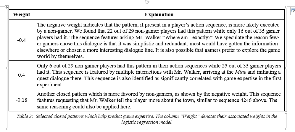
Before we proceed, we list a table of variables we will use:
| $latex n_{d,k}$ |
The number of times words in document $latex d$ are assigned to topic $latex k$ |
| $latex n_{k,w}$ |
The number of times word $latex w$ is assigned to topic $latex k$ |
| $latex n_{d,\cdot}$ |
The number of words in document $latex d$ |
| $latex n_{k,\cdot}$ |
The number of words belonging to topic $latex k$ |
Now let’s see how to calculate $latex p(\vec{z}, \vec{w}| \alpha, \beta) &s=2$:
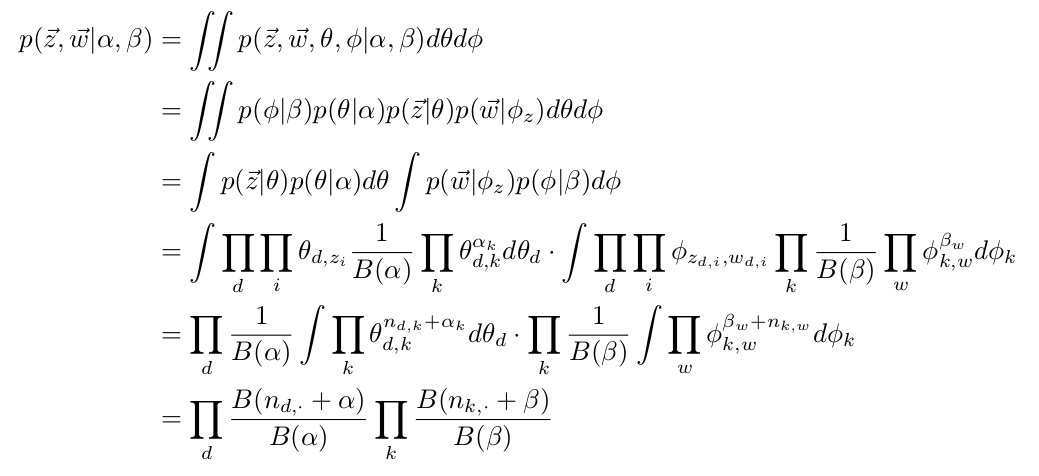
After that, we can have: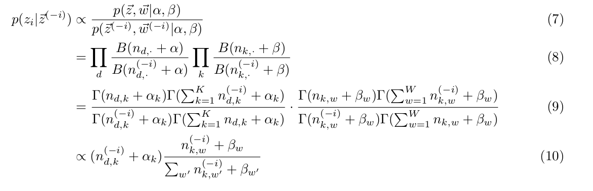
Among the equations above we applied the following properties:
1. For $latex \vec{\alpha} = (\alpha_1, \alpha_2, \dotsc, \alpha_K)$, $latex \vec{t}=(t_1, t_2, \dotsc, t_K)$ and $latex \sum_K t_i = 1 &s=2$:
$latex B(\vec{\alpha})=\frac{\prod^K_{i=1}\Gamma(\alpha_i)}{\Gamma(\sum^K_{i=1}\alpha_i)}=\int_0^1 t_i^{\alpha_i-1} d\vec{t} &s=2$
2. $latex \Gamma(n) = (n-1)!$
3. From (9) to (10), since we are sampling $latex z_i$ among 1 to K topics, so no matter which topic $latex z_i$ is, $latex \frac{\Gamma(\sum^K_{k=1}n_{d,k}^{(-i)}+ \alpha_k)}{\Gamma(\sum^K_{k=1}n_{d,k} + \alpha_k)} &s=3$ is always $latex \frac{1}{\sum_{k=1}^K n_{d,k}^{(-i)} + \alpha_k} &s=3$ which the Gibbs Sampler could ignore.
Till now, Gibbs Sampler knows everything it needs to calculate the conditional probability $latex p(z_i | \vec{z}^{(-i)}) $ by counting $latex n_{d,k} &s=2$, $latex n_{k,w} &s=2$, $latex n_{d,\cdot} &s=2$ and $latex n_{k,\cdot} &s=2$, and knowing $latex \alpha$ and $latex \beta$.
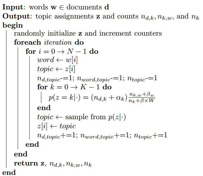
Pseudo-code
References
http://u.cs.biu.ac.il/~89-680/darling-lda.pdf
https://gist.github.com/mblondel/542786
http://blog.csdn.net/v_july_v/article/details/41209515
http://www.mblondel.org/journal/2010/08/21/latent-dirichlet-allocation-in-python/

 may have at most one other attribute as its parent other than the class variable
  . For example (figure from [1]):
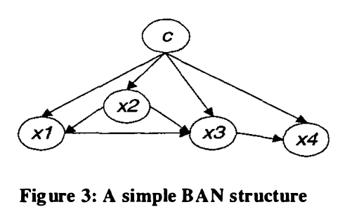
 , you start from a random network structure
  and calculate its
  . We set the current best network structure
  . Then for any other possible structure
  ,
,  if
if  . As you can see, we want to find a network structure which can minimize MDL(g|D).
 :
:
 given data
  comes into place to regulate the overall structure:
 is the number of parameters in the network.
  is the size of dataset.
  is the length of bits to encode every parameter. So
  has two possible values, i.e.,
  . Similarly,
  ,
,  ,
,  , and
, and  . Then attribute
  can have
  combinations of values. Further, we can use one more parameter to represent the joint probability of
  , one minus which is the joint probability of
  . Hence
  . Why we can use
  is replaced by mutual information format. Such transformation is equivalent and was proved in [4].
 number of the parameters in the network. This is exactly what I explained two paragraphs earlier.
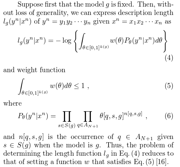
 is a vector of length
  . Each component of vector
 ![\theta[q,s,g]](https://czxttkl.com/wp-content/ql-cache/quicklatex.com-ba246c3dbb92dca4ba3457bb825a3593_l3.png "Rendered by QuickLaTeX.com") , which refers to the conditional probability of observing
, which refers to the conditional probability of observing  and
and  given a model
 ![\sum_{q}\sum_{s}\theta[q,s,g] =1](https://czxttkl.com/wp-content/ql-cache/quicklatex.com-10d362620c363ec91a63621edf3e193e_l3.png "Rendered by QuickLaTeX.com") .
. is the prior distribution of the vector
 . The real marginal probaiblity of
  is to integrate over all possible
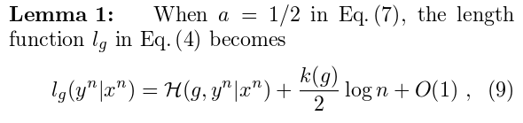
 is just to take negative log as in equation (4). I don’t quite get it at this point. What I can think of is that the negative log likelihood is perfect for its monotonically decreasing property. The higher probability of