BFGS and L-BFGS materials

Good explanation for BFGS and L-BFGS can be found in this textbook: https://www.dropbox.com/s/qavnl2hr170njbd/NumericalOptimization2ndedJNocedalSWright%282006%29.pdf?dl=0

In my own words:

Gradient descent and its various variants have been proved to learn parameters well in practical unconstrained optimization problems. However, it may converge too slowly or too roughly depending on how you set learning rate.

Remember the optimum in unconstrained optimization has zero first derivative. Newton (and Raphson) method uses tangent information of first derivative (i.e., second derivative) to find root of first derivative (i.e., the value making first derivative equal to zero). It usually converges in a quadratic convergence rate (if classic assumptions of Newton method are satisfied). However, in every iteration of Newton method for a multivariate unconstrained optimization, not only the Hessian matrix but its inversion need to be calculated, which prohibits from Newton method being applied to high dimension problems.

BFGS, as a member of quasi-Newton method family, uses cheaper calculation to approximate inversion of Hessian. But it is still expensive in respect of memory usage. Later, L-BFGS was coined to use thrift memory to achieve comparable precision as BFGS does.


My notes in implementing L-BFGS:

We use the same notation as in the textbook written by Jorge Nocedal:

Screenshot from 2016-01-03 14:37:18

You need to use line search to determine $latex \alpha_k$.  Simple backtracking line search is not going to work because $latex p_k$ should satisfy both Wolfie conditions.

Screenshot from 2016-01-03 14:39:12

Screenshot from 2016-01-03 14:40:19

People have designed different versions of line search to meet both Wolfie conditions (see: https://www.math.lsu.edu/~hozhang/papers/nonmonotone.pdf and https://github.com/JuliaOpt/Optim.jl/issues/26), I am using a simple version:

  1. if 3.6a is not satisfied, reduce $latex \alpha_k$ by half in every line search iteration.
  2. when 3.6a is satisfied, double $latex \alpha_k$ until 3.6b is satisfied.


When you determine $latex p_k$, you can also check if $latex \nabla(f_k) p_k = \nabla(f_k) H_k \nabla(f_k)> 0$. $latex H_k$ in every iteration in BFGS should be positive definite because:

H should be positive definite, so that f(x) reaches local minimum at $latex H^{-1} p$. 

https://en.wikipedia.org/wiki/Hessian_matrix#Second_derivative_test


Reference

http://www.alglib.net/optimization/lbfgsandcg.php

http://aria42.com/blog/2014/12/understanding-lbfgs/

http://andrew.gibiansky.com/blog/machine-learning/hessian-free-optimization/

http://papers.nips.cc/paper/5333-large-scale-l-bfgs-using-mapreduce.pdf

Recommendation System Review

Traditional Collaborative Filtering

  1. each user is represented by a O(N) length vector. N is the number of items.
  2. Therefore, user-item matrix has size O(MN). M is the number of users.
  3. for a user we want to recommend items for, we scan through user-item matrix, and find most similar k users.
  4. Based on the item vectors of the most similar k users, we recommend items.

cons: computationally expensive, since you need O(MN) in worst case to find the most similar k users.

Cluster Models

  1. similarly, construct a user-item matrix of O(MN) size
  2. cluster users into k groups
  3. for a user we want to recommend items for, we first identify which cluster he belongs to.
  4. Among the users in that cluster, we find items to recommend.

pros: for a user to be recommended, only O(k) time is needed to locate his desired cluster, thus reduces time complexity.

cons: The recommendation quality is not too good, given that users in the cluster are not the most similar users to the target user.

Search-Based Method

Search items with same author, artists, categories, etc of the item the target user just bought or rated. Then recommended.

cons: The recommendation quality is still not good, because a user’s next wanted items are not necessarily items with same author, artisits, categories, etc.

Item-to-Item Collaborative Filtering

  1. each item is represented by  a O(M) vector, which records which users have bought this item.
  2. construct a O(N^2) item-item matrix, M_{ij} is the similarity between item i and item j. This step runs offline. Worst case time complexity is O(N^2 M). But since the matrix should be very sparse, and it is computed offline, such time complexity is acceptable.
  3. When a target user buys an item, you can immediately find its most similar item and recommend it to the user.

Collaborative filtering in practice often outperforms content based filtering. However, collaborative filtering, either item based or user based, has a drawback: cold start problem. For new products/new user, its vector will not be well represented until a fair amount of time. Therefore,the quality of CF recommendation on the new product/user will downgrade. In light of this, content based filtering has its advantage. Another minor drawback of CF is its inability to recommend to users with unique taste.

Matrix Factorization Model

Each item and user is represented by a vector which describes the item’s or the user’s innate property. The dot product of a user vector \vec{p_u} \in \mathbb{R}^F and an item vector \vec{q_i} \in \mathbb{R}^F reflects how closely the two relate, where F, the dimension of the vector, will be determined by how granular you want to model user/item. As in the netflix prize competition, people reported to use 50-1500 dimensions. The higher the dimension they used, the better the recommendation quality reportedly.

The traditional matrix factorization model, such as SVD, can’t directly be applied to factorize user-item matrix because most of its elements are sparse. You can’t just simply zero an entry <i,j> in the user-item matrix.

There are many versions of matrix factorization model.

  1. In the scenarios where explicit feedbacks are available, we would like to approximate the dot product of \vec{q_i} and \vec{p_u} to the explicit rating from user u on item i. As given by this paper, the objective function to minimize is:
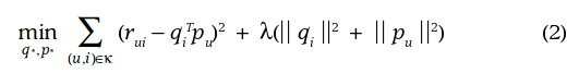
Screenshot from 2015-11-07 20:47:50where r_{ui} is the real rating from user u to item i.
  2. In many other scenarios, only implicit feedbacks are available. For example, each item is a TV show and r_{ui} denotes how long user u has watched the show. (unit: minutes). In this case, low r_{ui} indicates user u only watched a little portion of the show. But this can be due to many reasons intractable to capture: lack of interest, not perfect time for watching, laptop battery dying, etc. On the other hand, high r_{ui} indicates user u showed potentially strong interest in the show. Naturally, we want our objective function to accurately approximate strong r_{ui} but relax its rigorousness on approaching weak r_{ui}. Therefore, the approximation error, (r_{ui}-q_i^Tp_u)^2, should be weighted by a confidence parameter c_{ui} to give higher r_{ui} larger importance. c_{ui} can take various forms, such as c_{ui}= 1+\alpha r_{ui} or c_{ui} = 1+\alpha \log (1+r_{ui}/\epsilon).
  3. In implicit feedback scenario, there are two subcategories: ranking based and prediction based, each has its assumption. Ranking based learning algorithm assumes that implicit feedback difference, i.e., r_{ui}-r_{uj}, reflects the difference of the user’s interest between item i and j. Prediction based algorithm assumes there is a function p(r_{ui}) which binarizes r_{ui} which is more or less random/unpredictable/fluctuated. The approximation error thus becomes (p(r_{ui}) - q_i^T p_u)^2.

prediction based paper: http://yifanhu.net/PUB/cf.pdf

ranking based paper: http://wanlab.poly.edu/recsys12/recsys/p83.pdf

Learning for Matrix Factorization Model

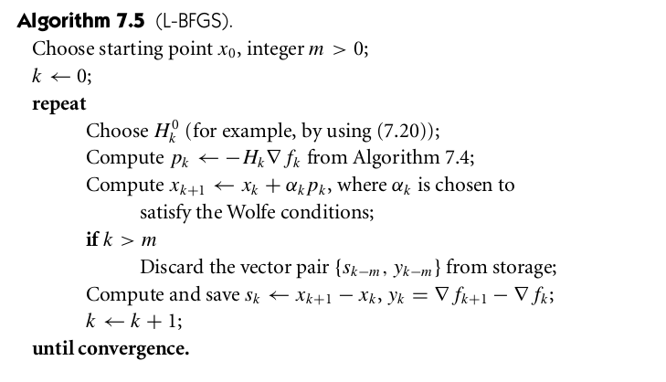
Stochastic gradient descent (SGD) or alternating least squares (ALS) can be used to learn parameters in the objective function. SGD is considered easier and faster but ALS can be parallelized on Mapreduce or Sparks. Both SGB and ALS’s time complexity is linear in the size of (user+item). This paper shows different parallelization strategies to learn matrix factorization model.

Bayesian Personalized Ranking Framework

A paper proposes a general Bayesian ranking framework which can be used for various recommendation system algorithm. The idea is to model the probability of observing every pair of items which user prefer differently (through implicit feedback), and maximize the joint probability of observing all such pairs w.r.t model specific parameters. Reading the paper’s section 4.3 will greatly help you understand the whole idea from its listed examples.

Incorporate temporal dynamics in Collaborative Filtering/Matrix Factorization

A more sophisticated model integrates temporal shift of user preference and item property in the recommendation. What they model in temporal aspect includes:

  1. user rating bias changes over time
  2. item rating bias (people tend to give higher/lower rating on certain items over others) changes over time
  3. For matrix factorization models, each component of the user vector (representing the user’s taste in a dimension) changes over time
  4. For collaborative filtering models, similarity between two items will be affected by time: if ratings for two items (i and j) from the same user happen within short time, their similarity should be high.

Finding candidate items to recommend

Once you have a trained model, the next thing is to give users recommendation. For collaborative filtering, you probably can immediately get most similar items for items a user just bought, depending on how you structure your data. For matrix factor models, you probably need more efforts to find a small set of candidate items, rather than the whole item set, and then determine the recommendation item within the candidate item subset. A stuff at Etcy reported that they used Locality-Similarity Hash (LSH) to find candidates. The item space is divided into subspaces by 2^k planes. Items falling into the same subspace constitute the candidate subsets.

Restricted Boltzmann Machines for Collaborative Filtering

It originates from a Geoffrey’s paper. (I felt hard to read.) Good tutorial about RBM can be found here: http://blog.echen.me/2011/07/18/introduction-to-restricted-boltzmann-machines/

The basic idea of RBM:

  1. Input layer is a binary vector of a user of length N, the total size of items. The number of hidden units is parameter and can be tuned.
  2. Based on the current weights and biases, predict hidden unit values.
  3. Based on the calculated hidden unit values, recalculate the input layer values
  4. The difference between the calculated input layer values and the observed input values is the objective function to minimize.
  5. All users share the same weights and biases.
  6. After the training process, for a new user with his own item vector, we can see which hidden units are activated hence determine his taste. Then, try to binary his taste at hidden units, and calculate input layer vector. Recommend any activated input unit that the user has not buy the corresponding item.

Deep learning

So far, I’ve only seen deep learning as resorts in content-based recommendation. One guy interned at Spotify reported using Convolutional Neural Network (CNN) on audio signals to extract features in order to contribute to Spotify’s recommendation system. Another guy who worked at Spotify used Recurrent Neural Network (RNN) to predict which track  a user will play next. The input to RNN will be user playing track history.

LDA in Recommendation System

fLDA is a model that borrows ideas from classic LDA model. It is suitable to the cases where meta-data of items are rich. It proposes that:
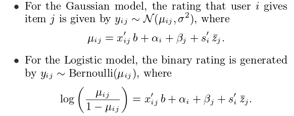
Screenshot from 2015-11-09 22:40:35

where x_{ij} is the user-item interaction vector, b is the weight vector for x_{ij}, \alpha_i is user i‘s bias variable, \beta_j is item j‘s bias variable, s_i is the user’s topic vector on k topics (representing the user’s interest on the k topics), and \bar{z_j} 
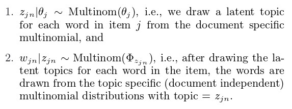
is the item’s topic soft clustering label.  \alpha_i, \beta_j and s_i are all random variables controlled by some forms of prior. \bar{z_j} is actually a mean of all words’ topic distribution in item j‘s meta data. The topic of a word in a item is generated in the following way as the same in classic LDA model:

Screenshot from 2015-11-09 22:51:06

Unlike classic LDA model such that z_{jn} is purely obtained from Collapsed Gibbs Sampling based upon text data, z_{jn} has also interaction with user topic vector s_i and hence determine his rating \mu_{ij}. Therefore, when sampling z_{jn} in the training process (E step), all ratings for the item the word belongs to will take into account:

Screenshot from 2015-11-10 00:03:21

That is why in the paper the authors mentioned that:

Screenshot from 2015-11-09 23:53:19

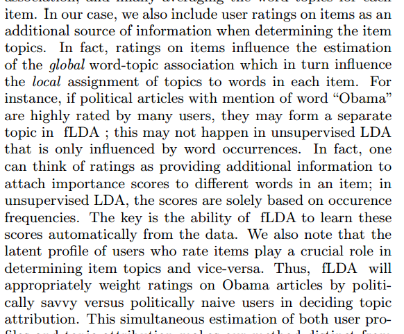
The training process is a bit intimidating as shown in the paper. Note that the authors claimed that the training process takes O(# of rating + # or words) time.

Other Tutorial Materials

A very complete recommendation system review tutorial can be found here, which was given by Xaiver Amatrian, previous research director at Netflix and now at Quora. Another tutorial is from Edwin Chen. An overview of content based recommendation approaches is given here. An overview of collaborative filtering methods can be found here. A good slide can be found here.

My Lempel-Ziv Compressor

Lempel-Ziv algorithm is a widely known compression algorithm. Its compression rate is proved to asymptotically reach the entropy of per symbol in the sequence to be compressed, when the length of the sequence is long enough.i.e., \frac{\text{compressed bits}}{\text{length of symbols } X_1 \cdots X_n } = H(X), where H(X) is per symbol entropy in the sequence X_1 \cdots X_n. If, for example, you have a sequence of letters of size n and each letter is encoded with 8 bits ASCII code, then the best compressed sequence also in ASCII will be of length \frac{H(X) \cdot n}{8}.

More details can be found in the classic information theory book written by Thomas & Cover.

I implemented my own Lempel-Ziv compressor/decompressor below. I intentionally challenged myself to write them as short as possible (perhaps in trade of readability).

Code

compress.py

import sys
from math import *

line = sys.stdin.readline()
i, b, d, res = 0, 0, {}, ''  # current pointer, block number,
                             # lookup table, return string
while i < len(line):
    for j in xrange(i+1, len(line)+1):
        if d.get(line[i:j]) is None or j == len(line):
            b += 1
            res += '{0:0{1}b}'.format(b-d.get(line[i:j-1], b), 
                int(ceil(log(b, 2)))) + line[j-1]
            d[line[i:j]] = b
            i, j = j, len(line)  # stop for-loop for j if cond1

sys.stdout.write(res[1:])    # strip prefix for first block

decompress.py

import sys
from math import *
 
line = sys.stdin.readline()
i, b, d, res = 0, 1, {}, ''     # current pointer, block number,
                                # lookup table, return string
while i < len(line):
	r = int(ceil(log(b, 2)))    # prefix range   
	code = d.get(b-int('0'+line[i:i+r], 2), '') + line[i+r]
	d[b] = code
	res += code
	i = i + r + 1
	b += 1

sys.stdout.write(res)

Usage (helper perl scripts and other related files can be downloaded here.):

# file.in contains "jaa"
# file.out contains the compressed code of "jaa"
# file.out1 contains the decompressed string of file.out, which is exactly "jaa".
# 0010100111000100101001111000110011000001
perl preCompress.pl < file.in | python compress.py | perl postCompress.pl > file.out
perl preDecompress.pl < file.out | python decompress.py | perl postDecompress.pl > file.out1

# Encode and decode my own name
echo -n 'zhc' | perl preCompress.pl | python compress.py | python decompress.py | perl postDecompress.pl

# Encode and decode random string
echo -n 'zasdfasdfasdlfasdlhc' | perl preCompress.pl | python compress.py | python decompress.py | perl postDecompress.pl

# Encode and decode files
perl preCompress.pl < alice.txt | python compress.py | perl postCompress.pl > alice.out
perl preDecompress.pl < alice.out | python decompress.py | perl postDecompress.pl > alice.out1

# Decode "CS6800"
echo -n 00110001101100011011100100111101110001010010011001100100011100100000000 | python decompress.py | perl postDecompress.pl

# Generate long sequence according to a markov chain (only three symbols)
python gen_mc.py > mc.in
# Compress long sequence generated according to markov chain
perl preCompress.pl < mc.in | python compress.py | perl postCompress.pl > mc_compressed.out
perl preDecompress.pl < mc_compressed.out | python decompress.py | perl postDecompress.pl > mc_decompressed.out1

Some observation

  1. The higher the per symbol entropy of the sequence is, the poorer the compression algorithm performs. I compressed a sequence containing only three symbols with around 30% compression rates. (The entropy per symbol is 1.459 bits/symbol) I also compressed a sequence of text (containing 26 English letters) from Alice Wonderland but with only 84% compression rate. As we know, the entropy of English letter should be much higher than 1.459 bits/symbol.
  2. I used real compressor such as `gzip` to compress my three symbol sequence, the compression rate is around 23%. As we know from the proved theory, the compression rate cannot be less than H(X)/8 = 1.459/8 = 18.2\%.

Graph Model Recap

I wrote a post before talking about sum-product algorithm: http://maider.blog.sohu.com/307377602.html

At that time, I had fresh memory on how graph model works. However, today when I read the post again, I am lost again. Therefore, I want to recap the basic motivations of graph models. This post can serve as an intro to the old post. I think remembering the motivations for an algorithm is really more important than details in it.

What does a Graph Model represent?

A graph model represents a joint distribution of all variables appearing in the a graph. There are three types of graph models, one is directed, one is undirected graph model, and the other is factor graph. For me, I find directed model is really intuitive because you can tell casual relationship from it. (See below the directed graph of the sex-gender-disease example I made in the sum-product algorithm post.) I am less familiar with undirected graph model, though. The factor graph is usually converted from directed/undirected graph model for inference learning purpose. So no matter what is your original graph model (directed or undirected), all learning algorithms take place at corresponding factor graphs.

A summary from Bishop’s book:

Screenshot from 2015-10-28 13:32:03

Another summary from his paper:

1 2 

Factor Graph

A factor graph consists of multiple factors, each is a clique connecting a fraction of total variables. Say you have want to calculate marginal distribution $latex p(x_i)$ from the joint distribution $latex p(x_1, x_2, \cdots, x_N)$. The naive way to calculate that is:

  1. get all possible configuration of $latex (x_1, x_2, \cdots, x_{i-1}, x_{i+1}, \cdots, x_N)$. 
  2. for each configuration $latex \hat{x}$, you calculate the joint probability of $latex p(x_i, \hat{x})$
  3. Sum all the joint probabilities under all configurations, which equals to $latex p(x_i)$.

If $latex x_1$ can take $latex |x_1|$ different values, $latex x_2$ can take $latex |x_2|$ different values, …, we will need to sum up $latex \prod\limits_{j \neq i} |x_j|$ joint probabilities.

Factor graph helps eliminate unnecessary computation. For example, if we have only four variables and the joint distribution is $latex p(x_1, x_2, x_3, x_4) = p(x_1)p(x_2|x_1)p(x_3|x_2)p(x_4|x_3) &s=2$, then $latex p(x_4)=\Big[\sum\limits_{x_3}p(x_4|x_3)\big[\sum\limits_{x_2}p(x_3|x_2)[\sum\limits_{x_1}p(x_1)p(x_2|x_1)]\big]\Big] &s=2$. Now you only need to compute addition operation $latex |x_1||x_2| + |x_2| + |x_3| $ times. 

What does Sum-Product algorithm do?

Sum-Product algorithm can easily calculate the marginal probability of any variable in the model. It, however, is not an inference learning algorithm. (i.e., it is not used for learning parameters in a graph model.)


What do inference algorithms do?

Inference algorithms learn the parameters of graph models. After that, you can use sum product algorithm to calculate marginal probability of any variable in the model. 


Use PDB to check variables before crashes

1. Use `python -i your_script.py` to execute your program with interactive mode. This means, after your program finishes executing, or your program crashes in the midway, you will enter a python shell.

2. Suppose your script has a bug so that you enter the python shell after it crashes. Now you can play with pdb by:

import pdb
pdb.pm()
# print your variables or do whatever you want


Leetcode 209: Minimum Size Subarray Sum

https://leetcode.com/problems/minimum-size-subarray-sum/

Minimum Size Subarray Sum

Total Accepted: 20591 Total Submissions: 84896 Difficulty: Medium

Given an array of n positive integers and a positive integer s, find the minimal length of a subarray of which the sum ≥ s. If there isn’t one, return 0 instead.

For example, given the array [2,3,1,2,4,3] and s = 7,
the subarray [4,3] has the minimal length under the problem constraint.

click to show more practice.

Credits:
Special thanks to @Freezen for adding this problem and creating all test cases.

Code 

import sys

class Solution(object):
    def minSubArrayLen(self, s, nums):
        """
        :type s: int
        :type nums: List[int]
        :rtype: int
        """
        p1 = p2 = 0
        cum = 0
        min_len = sys.maxint        

        for num in nums:
            cum += num
            if cum >=s:
                min_len = min(min_len, p1-p2+1)
                while p2 < p1:
                    if cum-nums[p2] >=s:
                        cum = cum-nums[p2]
                        p2 += 1
                        min_len = min(min_len, p1-p2+1)
                    else:
                        break
            p1 += 1

        return 0 if min_len == sys.maxint else min_len


Idea

Remember that all numbers are positive. You can have a fast pointer `p1` and a slow pointer `p2`. You first make the fast pointer to traverse the numbers until sum from nums[p2] to nums[p1] is more than s. Then, you start to move `p2` forward until the sum from nums[p2] to nums[p1] is no more than s anymore. In total, `p1` and `p2` both traverse at most O(N) distance. So the time complexity of the algorithm is O(N). Since we don’t require additional space, the space complexity of the alogrithm is O(1).


Leetcode 208: Implement Trie (Prefix Tree)

https://leetcode.com/problems/implement-trie-prefix-tree/

Implement Trie (Prefix Tree)

Total Accepted: 18703 Total Submissions: 75061 Difficulty: Medium

Implement a trie with insert, search, and startsWith methods.

Note:
You may assume that all inputs are consist of lowercase letters a-z.


Code

class TrieNode(object):
    def __init__(self):
        """
        Initialize your data structure here.
        """
        self.nodes = dict()
        self.is_word = False 


class Trie(object):

    def __init__(self):
        self.root = TrieNode()

    def insert(self, word):
        """
        Inserts a word into the trie.
        :type word: str
        :rtype: void
        """
        p = self.root
        for idx, ch in enumerate(word):
            if not p.nodes.get(ch, None):         
                p.nodes[ch] = TrieNode()
            p = p.nodes[ch]
            if idx==len(word)-1:
                p.is_word = True

    def search(self, word):
        """
        Returns if the word is in the trie.
        :type word: str
        :rtype: bool
        """
        p = self.root
        for idx, ch in enumerate(word):
            if not p.nodes.get(ch, None):
                return False
            p = p.nodes[ch]
            if idx==len(word)-1 and not p.is_word:
                return False
        
        return True
        

    def startsWith(self, prefix):
        """
        Returns if there is any word in the trie
        that starts with the given prefix.
        :type prefix: str
        :rtype: bool
        """
        p = self.root
        for idx, ch in enumerate(prefix):
            if not p.nodes.get(ch, None):
                return False
            p = p.nodes[ch]
            
        return True
        

# Your Trie object will be instantiated and called as such:
# trie = Trie()
# trie.insert("somestring")
# trie.search("key")


Idea

See idea about Trie:

http://www.geeksforgeeks.org/trie-insert-and-search/

https://leetcode.com/discuss/34840/maybe-the-code-is-not-too-much-by-using-next-26-c

Leetcode 220: Contains Duplicate III

https://leetcode.com/problems/contains-duplicate-iii/

Contains Duplicate III

Total Accepted: 15083 Total Submissions: 90517 Difficulty: Medium

Given an array of integers, find out whether there are two distinct indices i and j in the array such that the difference between nums[i] and nums[j] is at most t and the difference between i and j is at most k.

Code

import sys

class Solution(object):
    def containsNearbyAlmostDuplicate(self, nums, k, t):
        """
        :type nums: List[int]
        :type k: int
        :type t: int
        :rtype: bool
        """
        if not nums or k <=0 or t<0:
            return False

        def tran_num(org_num):
            return org_num + sys.maxint     
            
        def to_bucket(num_tran):
            return num_tran / (t+1)

        bucket_dict = {}
        for idx, num in enumerate(nums):
            num_tran = tran_num(num)
            bucket = to_bucket(num_tran)        
            
            if bucket_dict.get(bucket) or \
                bucket_dict.get(bucket+1, num_tran+t+1) - num_tran <=t or \
                num_tran - bucket_dict.get(bucket-1, num_tran-t-1) <=t:
                return True
                
            if idx >=k:
                old_bucket = to_bucket(tran_num(nums[idx-k]))
                bucket_dict.pop(old_bucket)
            
            bucket_dict[bucket] = num_tran

        return False


Idea (https://leetcode.com/discuss/38206/ac-o-n-solution-in-java-using-buckets-with-explanation)

We want to check if a number differs at most t with any of previous k elements by checking if any two numbers fall into the same bucket we shall create.

To do so, we first need to add every number by `sys.maxint`. This is to make sure every number can be transformed into an non-negative number so that we don’t need to worry about how to make different bucketing rules for negative and positive numbers.

For one transformed number, `num_tran`, we assign it to bucket `num_tran/(t+1)`. If two numbers fall into the same bucket, they must be of at most t difference. However, two numbers can also differ at most t if they are from two adjacent buckets. That’s why we have three condition checkings at line 25-27.

bucket_dict always has at most K elements. We maintain that by always popping out idx-k element. (line 30-32)

The time complexity is O(N) and the space complexity is O(K). 


Idea II

You can also maintain a balanced binary search tree of size K. Then you can always get the closest value of nums[i] (current visiting number) in the binary search tree in O(logK). If the closest value is within t of nums[i]’s range, you can return True.  Since you need to traverse all numbers in nums, and for each number you need to search in O(logK) time, the time complexity is O(NlogK) and the space complexity is O(K).

Reference:

https://leetcode.com/discuss/38177/java-o-n-lg-k-solution

Leetcode 261: Graph Valid Tree

https://leetcode.com/problems/graph-valid-tree/

Graph Valid Tree

Total Accepted: 2794 Total Submissions: 10778 Difficulty: Medium

Given n nodes labeled from 0 to n - 1 and a list of undirected edges (each edge is a pair of nodes), write a function to check whether these edges make up a valid tree.

For example:

Given n = 5 and edges = [[0, 1], [0, 2], [0, 3], [1, 4]], return true.

Given n = 5 and edges = [[0, 1], [1, 2], [2, 3], [1, 3], [1, 4]], return false.

Hint:

  1. Given n = 5 and edges = [[0, 1], [1, 2], [3, 4]], what should your return? Is this case a valid tree? Show More Hint

Note: you can assume that no duplicate edges will appear in edges. Since all edges are undirected, [0, 1] is the same as [1, 0] and thus will not appear together inedges.


Overall idea

We need to check two properties to determine whether a set of edges form a valid tree:

  1. it has n-1 edges
  2. it is acyclic


Code 1 (Union Find)

class Solution(object):
    def validTree(self, n, edges):
        """
        :type n: int
        :type edges: List[List[int]]
        :rtype: bool
        """
        union_arr = range(n)
        def find_union(p):
            if  union_arr[p] == p:
                return p
            else:
                return find_union(union_arr[p])        
                
        for p1, p2 in edges:
            p1_set = find_union(p1)        
            p2_set = find_union(p2)
            if p1_set == p2_set:
                return False
            union_arr[p1_set] = p2_set
        
        return len(edges) == n-1


Idea

This algorithm uses an idea called union find. You first initialize each node so that each node itself forms a node set. (We use `union_arr` to record which set a node belongs to).  As we traverse all edges, we will find connected components. The union find algorithm makes sure that every node in a connected component will point to a same node set by using `find_union` function. Therefore, if we see a new edge with two points in the same node set, we will return False because the edge makes a cycle in the graph.  If no cycle is found, we will finally check if there are exactly `n-1` edges to form a tree rather than disjoint parts in the graph. (line 22)

Reference

https://leetcode.com/discuss/52563/ac-java-union-find-solution

http://www.geeksforgeeks.org/union-find/


Updated 2016/09/30:

The union find algorithm can also be used to find connected components in an undirected graph. See leetcode 130: Surrounding Regions.


Code 2 (DFS)

class Solution(object):
    def validTree(self, n, edges):
        """
        :type n: int
        :type edges: List[List[int]]
        :rtype: bool
        """
        adj = {s:[] for s in range(n)}
        for p1, p2 in edges:
            adj[p1] += [p2]
            adj[p2] += [p1]
        stk = [0]
        while stk:
            cur = stk.pop()
            stk.extend(adj.pop(cur, []))
        return len(edges)==n-1 and not adj

Idea

We start to visit all nodes from node 0. (line 12) If we finish traversing all reachable nodes but there are still some adjacency matrix entry left then we know the given edges actually form multiple separate graphs. Therefore we should return False.


Code 3(BFS)

from collections import deque
class Solution(object):
    def validTree(self, n, edges):
        """
        :type n: int
        :type edges: List[List[int]]
        :rtype: bool
        """
        adj = {s:[] for s in range(n)}
        for p1, p2 in edges:
            adj[p1] += [p2]
            adj[p2] += [p1]
        q = deque()
        q.append(0)
        while q:
            cur = q.popleft()
            q.extend(adj.pop(cur, []))
        return len(edges)==n-1 and not adj


Idea

Similar idea as in code 2. But you implement the traversal of nodes using `deque`.