I haven’t learnt any new loss function for a long time. Today I am going to learn one new loss function, focal loss, which was introduced in 2018 [1].
Let’s start from a typical classification task. For a data ![]() , where
, where ![]() is the feature vector and
is the feature vector and ![]() is a binary label, a model predicts
is a binary label, a model predicts ![]() . Then the cross entropy function can be expressed as:
. Then the cross entropy function can be expressed as:
![]()
If you set

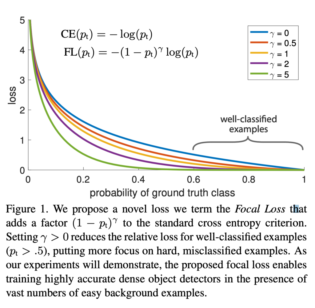
When there are many easy examples, i.e., p_t > 0.6 and the direction matches with the ground-truth label, the loss is small. However, if a dataset has an overwhelmingly large number of such easy examples as in the CV object detection domain, all these small losses add up to overwhelm the hard examples, i.e., those with p_t < 0.6.
Focal loss’s idea is to penalize losses for all kinds of examples, easy or hard, but the easy examples get penalized much more. Focal loss is defined as: ![]() . By tuning with different
. By tuning with different ![]() ‘s, you can see that the loss curve gets modulated differently and easy examples’ loss become less and less important.
‘s, you can see that the loss curve gets modulated differently and easy examples’ loss become less and less important.
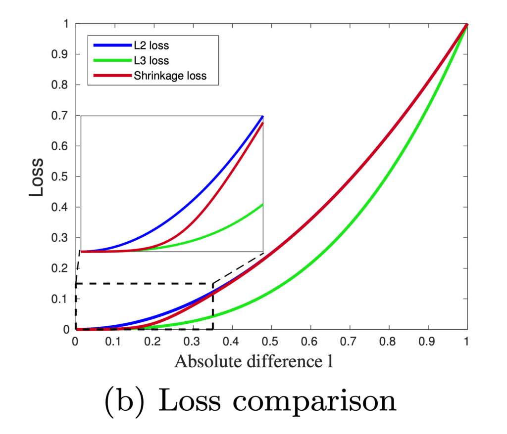
In the regression domain, we can define the MSE (L2) loss as below, with ![]() being the absolute prediction. error:
being the absolute prediction. error:
![]()
Applying the focal loss’s spirit on L_2, you get:
![]()
So the focal loss in the regression domain is just a higher-order loss.
[2] takes a step further on the ![]() by letting
by letting ![]() penalty effective almost only on the easy examples but not on the hard examples. They call it the shrinkage loss:
penalty effective almost only on the easy examples but not on the hard examples. They call it the shrinkage loss:
![Rendered by QuickLaTeX.com \[L_S = \frac{l^2}{1 + exp\left(a\cdot \left( c-l \right)\right)}\]](https://czxttkl.com/wp-content/ql-cache/quicklatex.com-60f04910d6082a4a6a347f51491eeac0_l3.png)

Reference
[1] Focal Loss for Dense Object Detection: https://arxiv.org/pdf/1708.02002.pdf
[2] Deep Regression Tracking with Shrinkage Loss: https://openaccess.thecvf.com/content_ECCV_2018/papers/Xiankai_Lu_Deep_Regression_Tracking_ECCV_2018_paper.pdf
The article introduces the focal loss, a loss function used in classification tasks, particularly for addressing the issue of overwhelming easy examples in datasets like object detection in computer vision. Focal loss penalizes losses for all examples, but easy examples are penalized more, helping to address class imbalance in certain tasks.