TRPO, PPO, Graph NN + RL

Writing this post to share my notes on Trust Region Policy Optimization [2], Proximal Policy Optimization [3], and some recent works leveraging graph neural networks on RL problems.

We start from the objective of TRPO. The expected return of a policy is $\eta(\pi)=\mathbb{E}_{s_0, a_0, \cdots}[\sum\limits_{t=0}^{\infty}\gamma^t r(s_t)]$ . The return of another policy $\hat{\pi}$ can be expressed as $\eta(\pi)$ and a relative difference term: $\eta(\hat{\pi})=\eta(\pi) + \sum\limits_s \rho_{\hat{\pi}}(s)\sum\limits_a \hat{\pi}(a|s) A_{\pi}(s,a)$ , where for any given $\pi$ , $\rho_{\pit}(s)=P(s_0) + \gamma P(s_1=s) + \gamma^2 P(s_2=s) + \cdots$ is called discounted state visitation frequency.

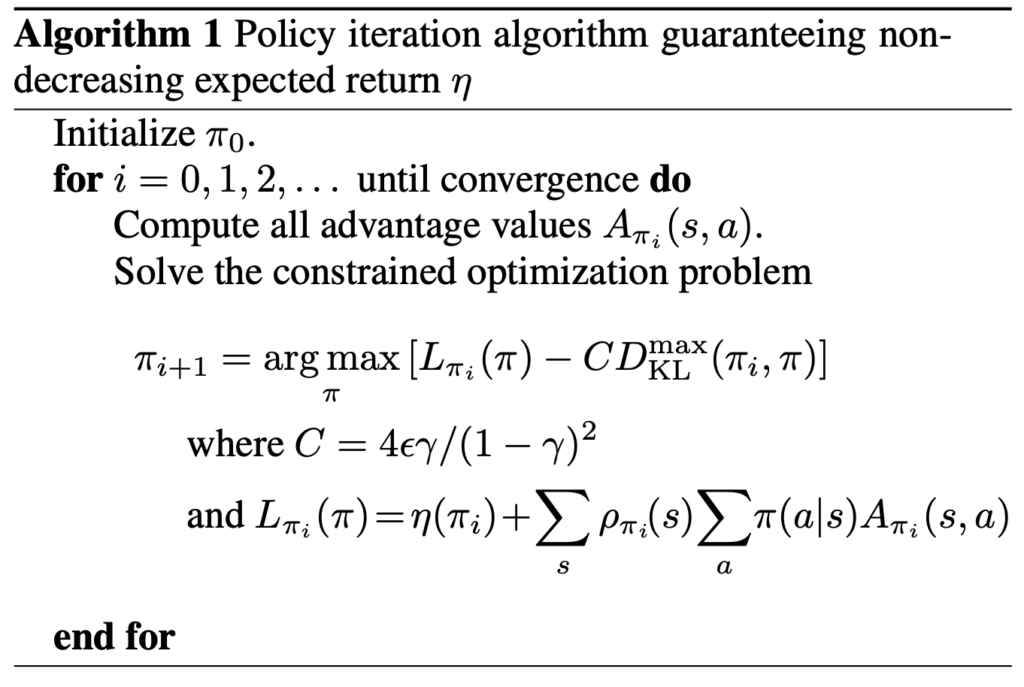
To facilitate the optimization process, the authors propose to replace $\rho_{\hat{\pi}}(s)$ with $\rho_{\pi}(s)$ . If the new policy $\hat{\pi}$ is close to $\pi$ , this approximation is not that bad since the discounted state visitation frequency shouldn’t change too much. Thus $\eta(\hat{\pi}) \approx L_{\pi}(\hat{\pi})=\eta(\pi) + \sum\limits_s \rho_{\pi}(s)\sum\limits_a \hat{\pi}(a|s)A_{\pi}(s,a)$ .

Using some theorem (See section 3 [2]) we can prove that $\eta(\hat{\pi}) \geq L_{\pi}(\hat{\pi})-C \cdot D^{max}_{KL}(\pi, \hat{\pi})$ , where $C=\frac{4\epsilon\gamma}{(1-\gamma)^2}$ , $\epsilon=max_{s,a}|A_{\pi}(s,a)|$ , and $D^{max}_{KL}(\pi, \hat{\pi})=\max_s D_{KL}(\pi(\cdot|s) \| \hat{\pi}(\cdot|s))$ . The inequality-equality becomes just equality if $\hat{\pi}=\pi$ . Therefore, $\arg\max_{\hat{\pi}}[L_{\pi}(\hat{\pi})-C\cdot D^{max}_{KL}(\pi, \hat{\pi})] \geq L_{\pi}(\pi)-C\cdot D^{max}_{KL}(\pi, \pi)=L_{\pi}(\pi)$ . Therefore, we can use algorithm 1 to monotonically improve $\pi$ .

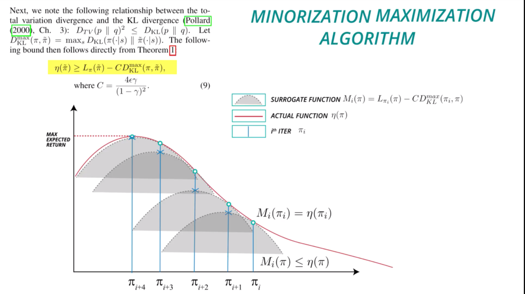
The algorithm 1 can also be understood through the diagram below (from [10]), where we set $M_i(\pi)=L_{\pi_i}(\pi)-CD^{max}_{KL}(\pi_i, \pi)$ .

In practice, we parameterize a policy with $\theta$ , and we move the coefficient $C$ from the objective to a constraint (the paper argues this could improve the policy in larger steps), and finally we use the average KL divergence between two policies rather than $D^{max}_{KL}$ . Putting these practical treatments together, we get:

$\arg\max\limits_{\theta} L_{\pi_{\theta_{old}}}(\pi_{\theta})=\sum\limits_s \rho_{\pi_{\theta_{old}}}(s)\sum\limits_a \pi_\theta(a|s)A_{\pi_{\theta_{old}}}(s,a) \newline \text{subject to } \bar{D}^{\rho_{\pi_{\theta_{old}}}}_{KL}(\pi_{\theta_{old}}, \pi_{\theta})\leq \delta$

If changing the sum to expectation $\mathbb{E}_{s\sim \rho_{\theta_{old}}, a\sim \pi_{\theta_{old}}}$ , we will need some importance-sampling re-weighting. And in practice, we can estimate Q-values from trajectories more easily than estimating advantages because we would need exhaust all actions at each step to compute advantages. Thus the objective function using empirical samples eventually becomes:

$\arg\max\limits_{\theta} \mathbb{E}_{s\sim \rho_{\pi_{\theta_{old}}}, a\sim \pi_{\theta_{old}}} \big[\frac{\pi_{\theta}(a|s)}{\pi_{\theta_{old}}(a|s)} Q_{\pi_{\theta_{old}}}(s,a)\big] \newline \text{subject to } \mathbb{E}_{s\sim \rho_{\pi_{\theta_{old}}}} \big[D_{KL}(\pi_{\theta_{old}}(\cdot|s) \| \pi_{\theta}(\cdot|s))\big]\leq \delta$

Suppose the objective is $f(\theta)=\frac{\pi_{\theta}(s|a)}{\pi_{\theta_{old}}(a|s)} Q_{\pi_{\theta_{old}}}(s,a)$ . Using Taylor series expansion, we have $f(\theta) \approx f(\theta_{old}) + \nabla_\theta f(\theta)|_{\theta=\theta_{old}}(\theta-\theta_{old})=f(\theta_{old}) + g^T (\theta-\theta_{old})$ . $f(\theta_{old})$ can be seen as a constant and thus can be ignored during optimization.

And for the constraint, we can also use Taylor series expansion (this is a very common trick to convert KL divergence between two distributions into Taylor series expansion). Suppose $h(\theta)=D_{KL}(\pi_{\theta_{old}}(\cdot|s) \| \pi_{\theta}(\cdot|s))$ , then $h(\theta)\approx h(\theta_{old}) + \nabla_\theta h(\theta) |_{\theta=\theta_{old}} (\theta-\theta_{old})+\frac{1}{2}(\theta-\theta_{old})^T \nabla^2_\theta h(\theta)|_{\theta=\theta_{old}}(\theta-\theta_{old})$ . We know that $h(\theta_{old})=0$ because it is the KL divergence between the same distribution $\pi_{\theta_{old}}$ . We can also know that $\nabla_\theta h(\theta) |_{\theta=\theta_{old}}=0$ because the minimum of KL divergence is 0 and is reached when $\theta=\theta_{old}$ hence the derivative at $\theta_{old}$ must be 0.

Removing all constant and zero terms, and with two more notations $s=\theta-\theta_{old}$ and $H=\nabla^2_\theta h(\theta)|_{\theta=\theta_{old}}$ , we rewrite the objective function as well as the constraint:

$\arg\min\limits_{s} -g^T s \newline\text{ subject to } \frac{1}{2}s^T H s - \delta \leq 0$

Now the Lagrange Multiplier optimization kicks in. Intuitively, the direction to get to the next $\theta$ is on the direction that minimizes $-g^T s$ while stretching the constraint by the most extent (at the moment when the equality of the constraint holds). Denote the Lagrange Multiplier as $\lambda$ (a single scalar because we only have one constraint) and the auxiliary objective function as $\mathcal{L}(s, \lambda)=-g^T s + \lambda (\frac{1}{2}s^T H s - \delta)$ . From Karush-Kuhn-Tucker (KTT) conditions, we want to find a unique $\lambda^*$ and the local minimum solution $s^*$ such that:

$\nabla_s \mathcal{L}(s^*,\lambda^*)=0$
$\lambda^* \geq 0$
$\lambda^*\cdot (\frac{1}{2}s^T H s - \delta) = 0$
$\frac{1}{2}s^{*T} H s^* - \delta \leq 0$ (actually, the equality should hold because $s^*$ should be obtained at the border of the constraint, although I am not sure how to prove it. This means, as long as we find some non-negative $\lambda^*$ such that $\nabla_s \mathcal{L}(s^*,\lambda^*)=0$ , the first four conditions are satisfied.)
$\nabla^2_s \mathcal{L}(x^*, \lambda^*)$ is positive semi-definite. $\nabla^2_s \mathcal{L}(x^*, \lambda^*)$ is just $H$ times some constant term. And we know from the fact that: (1) $H$ is the Fisher information matrix because it is the Hessian of KL divergence [12]; (2) a Fisher information matrix is positive semi-definite [13].

Since we don’t have analytical solution for $\frac{1}{2}s^{*T} H s^* - \delta = 0$ , we can’t know $s^*$ easily. We can start from looking at $\nabla_s \mathcal{L}(s^*,\lambda^*)=-g + \lambda^* Hs^* = 0$ . Moving $-g$ to the right side, we have $\lambda^* H s^*=g$ . Here, both $s^*$ and $\lambda^*$ are unknown to us. But we know that $s^*=\lambda^{*-1}H^{-1}g$ . Therefore, $s^*$ must be in the direction of $H^{-1}g$ . How to compute $H^{-1}g$ ? If we just compute $H^{-1}$ as pure matrix inversion, we would need $O(n^3)$ time complexity where $n$ is width/height of $H$ . Instead, we can first obtain the solution $x$ of the equation $H x=g$ using Conjugate Gradient Method; $x$ will be exactly $H^{-1}g$ . We will spend one section below to introduce Conjugate Gradient method but for now just remember Conjugate Gradient method can compute $x$ much faster than $O(n^3)$ as in matrix inversion. Back to our focus: once we get $H^{-1}g$ , we will try to take the step size $\beta$ that makes the constraint equality hold: $\frac{1}{2} \beta x^T H \beta x - \delta=0$ . Thus the $\beta$ would be obtained at $\beta=\sqrt{(\frac{2\delta}{x^T H x})}$ . Therefore, $\theta = \theta_{old}+\beta x$ . This is exactly one iteration of TRPO update!

We now introduce what the conjugate gradient method is, which is used to find the update direction in TRPO.

Conjugate Gradient Method

My summary is primarily based on [6]. CG is an iterative, efficient method to solve $Ax=b$ , which is the solution of the quadratic form $argmin_x f(x)=argmin_x \frac{1}{2}x^TAx-b^Tx+c$ . The most straightforward way to solve $Ax=b$ is to compute $A^{-1}$ and let $x=A^{-1}b$ . However, computing $A^{-1}$ needs $O(n^3)$ time complexity by Gaussian elimination method, where $n$ is the width (or height) of $A$ .

If we can’t afford to compute $A^{-1}$ , the best bet is to rely on iterative methods. We list some notations used across iterative methods before we proceed. The error $e_i=x_i - x$ is the distance between the i-th solution $x_i$ and the real solution $x$ . The residual $r_i=-f'(x_i)=b-Ax_i$ indicates how far we are from $b$ .

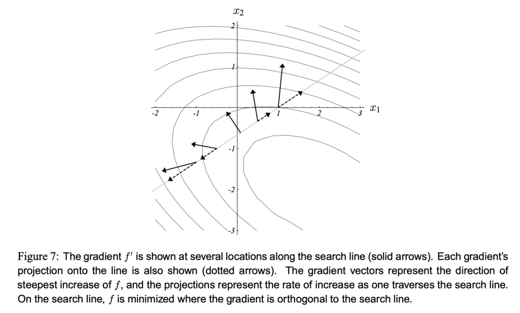
Steepest gradient descent with line search works as follows. At solution $x_i$ , take a step on the direction of $r_i$ , and the step size is determined such that the arrival point after the step, which is $x_{i+1}$ , should have the smallest $f(x_{i+1})$ . This can also be understood as $r_{i+1}$ should be orthogonal to $r_i$ . The two pictures below help illustrate the idea:

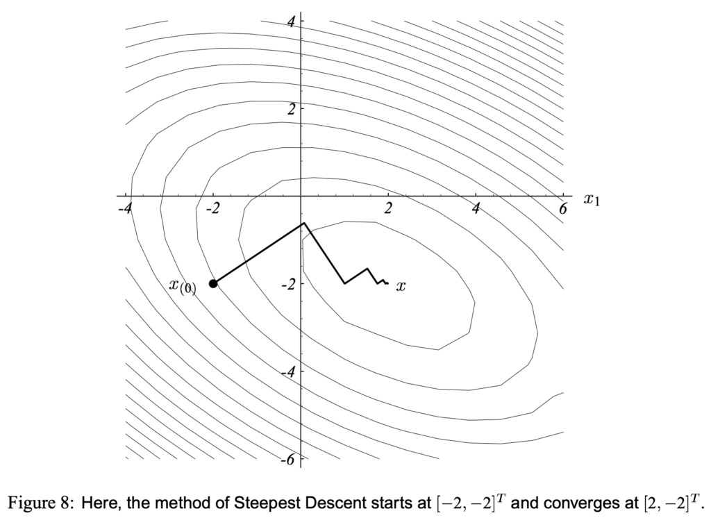
As you can see, the steepest gradient method often takes a zig-zag path to reach the sufficient proximity of the optimal solution. From theories (Section 6.2 in [6]), the number of steps it needs depends on the condition number of $A$ and the starting point $x_0$ . And from the intuition, the number of steps is no smaller than the number of bases of the solution space. The luckiest situation is that you pick $x_0$ which results to all orthogonal steepest gradients in the following steps. Such $x_0$ can also be thought to have $e_o$ parallel with any of the eigenvectors of $A$ :

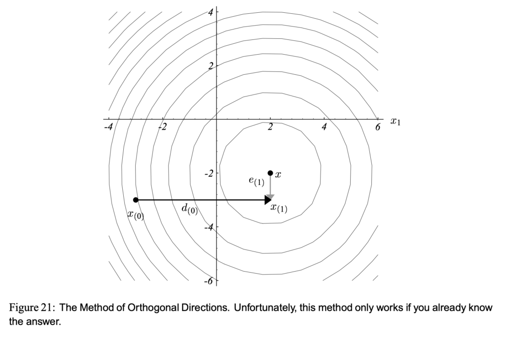
The idea of conjugate direction methods (conjugate gradient is one of conjugate direction methods) is to enforce the iterations happen exactly $n$ times to reach the optimal solution, where, by our definition, $n$ is the width (or height) of $A$ and also the number of bases of the solution space.

The procedure of conjugate direction methods starts from finding $d_0, d_1, \cdots, d_{n-1}$ search directions. If $d_0, d_1, \cdots, d_{n-1}$ can be orthogonal to each other, we can easily approach $x$ in $n$ steps, as in Figure 21. But theoretically we are not able to find such $n$ search directions. Instead, we can use Gram-Schmidt Conjugation and $u_0, u_1, \cdots, u_{n-1}$ linearly independent vectors to construct $n$ $A$ -orthogonal search directions. And it is provable that using $n$ $A$ -orthogonal search directions we can also approach $x$ in $n$ steps. However, for arbitrary $u_0, u_1, \cdots, u_{n-1}$ Gram-Schmidt Conjugation requires $O(n^2)$ space and $O(n^3)$ time complexity, which is a disadvantage in practice.

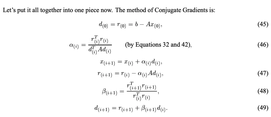
The method of conjugate gradients refers to the conjugate direction method when $u_0, u_1, \cdots, u_{n-1}$ are actually residuals $r_0, r_1, \cdots, r_{n-1}$ . Fortunately, it has a nice property that space complexity and time complexity can be reduced to $O(mn)$ , where $m$ is the number of nonzero entries of $A$ . Conjugate gradient can be summarized as follows:

Once you understand TRPO, PPO is much easier to be understood. PPO just simplifies the constrained optimization in TRPO to an unconstrained optimization problem. The main objective function of PPO is:

$L^{CLIP}\newline=CLIP\left(\mathbb{E}_{s\sim \rho_{\pi_{\theta_{old}}}, a\sim \pi_{\theta_{old}}} \left[\frac{\pi_{\theta}(a|s)}{\pi_{\theta_{old}}(a|s)} A_{\pi_{\theta_{old}}}(s,a)\right]\right)\newline=CLIP\left(\mathbb{E}_{s\sim \rho_{\pi_{\theta_{old}}}, a\sim \pi_{\theta_{old}}} \left[r(\theta)A_{\pi_{\theta_{old}}}(s,a)\right]\right)\newline=\mathbb{E}_{s\sim \rho_{\pi_{\theta_{old}}}, a\sim \pi_{\theta_{old}}} \left[min(r(\theta), clip(r(\theta), 1-\epsilon, 1+\epsilon)) \cdot A_{\pi_{\theta_{old}}}(s,a)\right]$

Let’s understand this clipped objective by some example. If $A_{\pi_{\theta_{old}}}(s,a)$ is positive, the model tries to increase $r(\theta)$ but no more than $1+\epsilon$ ; if $A_{\pi_{\theta_{old}}}(s,a)$ is negative, the model tries to decrease $r(\theta)$ but no less than $1-\epsilon$ . This way, the change of the policy is limited.

Now, let me examine the paper [5], because of which I started investigating TRPO and PPO. [5] models each joint in a robot in a locomotion task as a node in a graph. In graph learning, each node is represented as an embedding. At any given time step, the state feature can be summarized by all nodes’ embeddings. In [5], the policy network is learned through PPO.

[4] uses graph learning to model job scheduling graphs. But they use REINFORCE to learn their policy because their actions are defined as selecting one node out of all available nodes for scheduling.

Besides using graph learning to encode a graph into some feature representation, I’ve also seen people using tree-LSTM to encode tree-like graphs [14].

Reference

[1] Spinning Up doc about TRPO: https://spinningup.openai.com/en/latest/algorithms/trpo.html

[2] Trust Region Policy Optimization: https://arxiv.org/abs/1502.05477

[3] Proximal Policy Optimization Algorithms: https://arxiv.org/abs/1707.06347

[4] Learning Scheduling Algorithms for Data Processing Clusters: https://arxiv.org/abs/1810.01963

[5] NerveNet: Learning Structured Policy with Graph Neural Networks: https://openreview.net/pdf?id=S1sqHMZCb

[6] An Introduction to the Conjugate Gradient Method Without the Agonizing Pain: https://www.cs.cmu.edu/~quake-papers/painless-conjugate-gradient.pdf

[7] CS294-112 10/11/17: https://www.youtube.com/watch?v=ycCtmp4hcUs&feature=youtu.be&list=PLkFD6_40KJIznC9CDbVTjAF2oyt8_VAe3

[8] Towards Data Science PPO vs. TRPO: https://towardsdatascience.com/introduction-to-various-reinforcement-learning-algorithms-part-ii-trpo-ppo-87f2c5919bb9

[9] Efficiently Computing the Fisher Vector Product in TRPO: http://www.telesens.co/2018/06/09/efficiently-computing-the-fisher-vector-product-in-trpo/

[10] TRPO (Trust Region Policy Optimization) : In depth Research Paper Review: https://www.youtube.com/watch?v=CKaN5PgkSBc

[11] Optimization Overview: https://czxttkl.com/2016/02/22/optimization-overview/

[12] https://wiseodd.github.io/techblog/2018/03/14/natural-gradient/

[13] https://stats.stackexchange.com/questions/49942/why-is-the-fisher-information-matrix-positive-semidefinite

[14] Learning to Perform Local Rewriting for Combinatorial Optimization https://arxiv.org/abs/1810.00337

Dropbox Download

TRPO, PPO, Graph NN + RL

Leave a comment

Cancel reply