DPG and DDPG

In this post, I am sharing my understanding regarding Deterministic Policy Gradient Algorithm (DPG) [1] and its deep-learning version (DDPG) [2].

We have introduced policy gradient theorem in [3, 4]. Here, we briefly recap. The objective function of policy gradient methods is:

$J(\theta)=\sum\limits_{s \in S} d^\pi(s) V^\pi(s)=\sum\limits_{s \in S} d^\pi(s) \sum\limits_{a \in A} \pi(a|s) Q^\pi(s,a),$

where $\pi$ represents $\pi_\theta$ , $d^\pi(s)$ is the stationary distribution of Markov chain for $\pi$ , $V^\pi(s)=\mathbb{E}_{a \sim \pi}[G_t|S_t=s]$ , and $Q^{\pi}(s,a)=\mathbb{E}_{a \sim \pi}[G_t|S_t=s, A_t=a]$ . $G_t$ is accumulated rewards since time step $t$ : $G_t=\sum^\infty_{k=0}\gamma^k R_{t+k}$ .

Policy gradient theorem proves that the gradient of policy parameters with regard to $J(\theta)$ is:

$\nabla_\theta J(\theta) = \mathbb{E}_{\pi}[Q^\pi(s,a)\nabla_\theta ln \pi_\theta(a|s)]$

More specifically, the policy gradient theorem we are talking about is stochastic policy gradient theorem because at each state the policy outputs a stochastic action distribution $\pi(s|a)$ .

However, the policy gradient theorem implies that policy gradient must be calculated on-policy, as $\mathbb{E}_{\pi}:=\mathbb{E}_{s\sim d^{\pi}, a\sim \pi}$ means the state and action distribution is generated by following $\pi_\theta$ .

If the training samples is generated by some other behavioral policy $\beta$ , then the objective function becomes:

$J(\theta)=\sum\limits_{s \in S} d^\beta(s) V^\pi(s)=\sum\limits_{s \in S} d^\beta(s) \sum\limits_{a \in A} \pi(a|s) Q^\pi(s,a),$

and we must rely on importance sampling to calculate the policy gradient [7,8]:

$\nabla_\theta J(\theta) = \mathbb{E}_{s\sim d^\beta}[\sum\limits_{a\in A}\nabla_\theta \pi(a|s) Q^\pi(s,a) + \pi(a|s)\nabla_\theta Q^\pi(s,a)] \newline \approx \mathbb{E}_{s\sim d^\beta}[\sum\limits_{a\in A}\nabla_\theta \pi(a|s) Q^\pi(s,a)] \newline =\mathbb{E}_{\beta}[\frac{\pi_\theta(a|s)}{\beta(a|s)}Q^\pi(s,a)\nabla_\theta ln \pi_\theta(a|s)]$

where $\mathbb{E}_{\beta}:=\mathbb{E}_{s\sim d^\beta, a\sim\beta}$

However, using importance sampling $\frac{\pi_\theta(a|s)}{\beta(a|s)}$ could incur some learning difficulty problems [5]:

Screen Shot 2019-01-23 at 6.31.41 PM

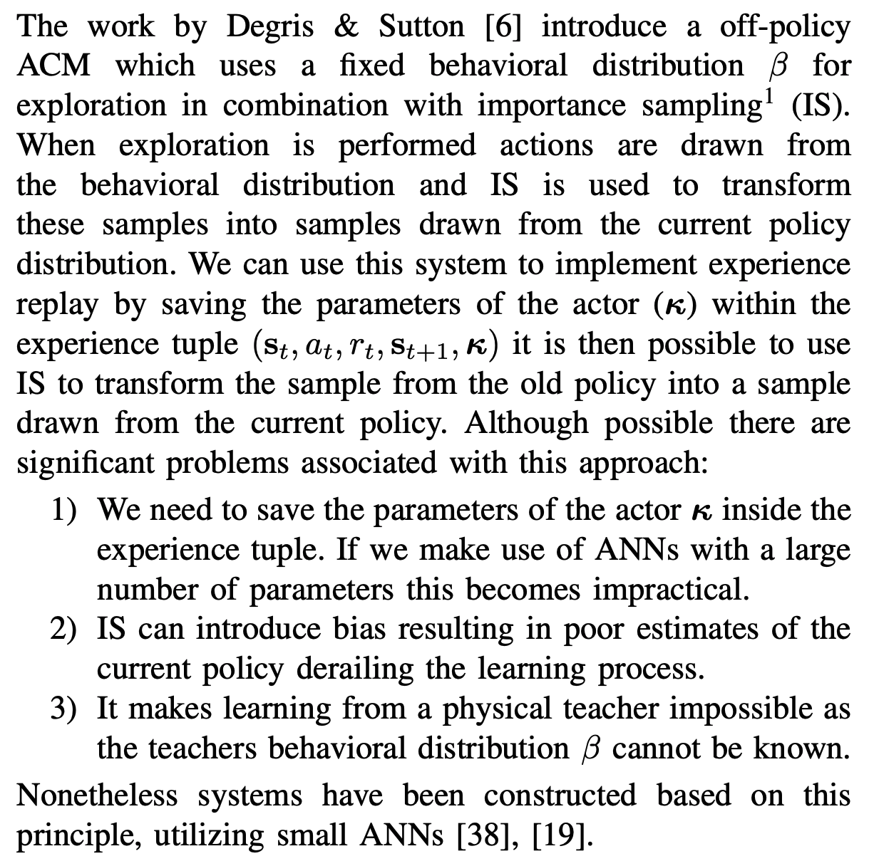
What DPG proposes is that we design a policy that outputs actions deterministically: $a = \mu_\theta(s)$ , thus $J(\theta)$ would only have integration (or sum) over state distribution and get rid of importance sampling, which makes learning potentially easier:

$J(\theta)=\sum\limits_{s \in S} d^\beta(s) V^\mu(s)=\sum\limits_{s \in S} d^\beta(s) Q^\mu(s, \mu_\theta(s))$

Writing the above formula in integration (rather than discrete sum), we get:

$J(\theta)=\int\limits_S d^\beta(s) V^\mu(s) ds=\int\limits_{S} d^\beta(s) Q^\mu(s, \mu_\theta(s)) ds$

And the gradient of $J(\theta)$ is:

$\nabla_\theta J(\theta) = \int\limits_S d^\beta(s) \nabla_\theta Q^\mu(s, \mu_\theta(s)) ds \approx \mathbb{E}_\beta [\nabla_\theta \mu_\theta(s) \nabla_a Q^\mu(s,a)|_{a=\mu_\theta(s)}]$

This immediately implies that $\theta$ can be updated off policy. Because we only need to sample $s \sim d^\beta(s)$ , then $\nabla J(\theta)$ can be calculated without knowing what action the behavior policy $\beta$ took (we only need to know what the training policy would take, i.e., $a=\mu_\theta(s)$ ). We should also note that there is an approximation in the formula of $\nabla_\theta J(\theta)$ , because $\nabla_\theta Q^u(s,\mu_\theta(s))$ cannot be applied chain rules easily since even you replace $\mu_\theta(s))$ with $a$ , the $Q$ function itself still depends on $\theta$ .

Updating $\theta$ is one part of DPG. The other part is fitting a Q-network with parameter $\phi$ on the optimal Q-function of policy governed by $\theta$ . This equates to update according to mean-squared Bellman error (MSBE) [10], which is the same as in Q-Learning.

I haven’t read the DDPG paper [2] thoroughly but based on my rough understanding, it adds several tricks when dealing with large inputs (such as images). According to [9]’s summary, DDPG introduced three tricks:

add batch normalization to normalize “every dimension across samples in one minibatch”
add noise in the output of DPG such that the algorithm can explore
soft update target network

References

[1] Silver, D., Lever, G., Heess, N., Degris, T., Wierstra, D., & Riedmiller, M. (2014, June). Deterministic policy gradient algorithms. In ICML.

[2] Lillicrap, T. P., Hunt, J. J., Pritzel, A., Heess, N., Erez, T., Tassa, Y., … & Wierstra, D. (2015). Continuous control with deep reinforcement learning. arXiv preprint arXiv:1509.02971.

[3] Notes on “Soft Actor-Critic: Off-Policy Maximum Entropy Deep Reinforcement Learning with a Stochastic Actor”: https://czxttkl.com/?p=3497

[4] Policy Gradient: https://czxttkl.com/?p=2812

[5] https://repository.tudelft.nl/islandora/object/uuid:682a56ed-8e21-4b70-af11-0e8e9e298fa2?collection=education

[6] https://stackoverflow.com/questions/42763293/what-is-the-advantage-of-deterministic-policy-gradient-over-stochastic-policy-gr

[7] https://lilianweng.github.io/lil-log/2018/04/08/policy-gradient-algorithms.html#off-policy-policy-gradient

[8] Degris, T., White, M., & Sutton, R. S. (2012). Off-policy actor-critic. arXiv preprint arXiv:1205.4839.

[9] https://lilianweng.github.io/lil-log/2018/04/08/policy-gradient-algorithms.html#ddpg

[10] https://spinningup.openai.com/en/latest/algorithms/ddpg.html#the-q-learning-side-of-ddpg